

6. ENVIRONMENTAL AND SOCIAL IMPACT ASSESSMENT
6.1 Introduction
The Environmental and Social Impact Assessment (ESIA) is a planning process that has become common practice for water storage infrastructure projects. In addition to an ESIA being a legal requirement, past experience has proven that proper public consultation and analysis of potential environmental and social impacts improves the likelihood of sustainable benefits from the project to a wider body of stakeholders and reduces the likelihood of negative impacts of the project on the social and bio-physical environment.
The construction of small dams, pans and other small scale water storage structures usually pose a smaller risk of adverse social and environmental impacts than the construction of large-scale dams and reservoirs. The ESIA process, scaled suitably to the scale and nature of the project in question, however remains an important component of project development particularly where fragile environments and vulnerable people are involved. For example in the case of arid and semi-arid areas, which are characterized by relatively limited surface water resources, care should be taken to ensure that the construction or rehabilitation of a small dam or pan does not upset delicate balances between quantity of water available, existing water uses and sustainable rangeland utilisation.
It is therefore important to note that the exploitation of (surface) water resources by the creation of an artificial reservoir, however limited in size, still constitutes an intervention in the hydrological cycle. It is therefore important that the social and environmental impacts be taken into account and addressed accordingly during the planning process.
This chapter provides an outline of the ESIA methodology as it applies to dams, pans and other water conservation structures. Readers should refer to other documents for a more comprehensive discussion on the ESIA process. The reader is also advised to review the material in Chapter 4 on Legal Compliance which presents the legal aspects of the ESIA process.
6.2 What is an ESIA
Design and construction of water storage structures is primarily informed by the opportunities for benefits associated with such a structure. But like any other infrastructure project, water storage structure projects also have the potential to trigger negative social and bio-physical impacts.
The Environmental and Social Impact Assessment (ESIA) is thus a project planning process that identifies, predicts and assesses the type and scale of potential social and bio-physical impacts and opportunities for benefits associated with the proposed water storage project.
The ESIA documents the baseline condition and how this is likely to change during construction, operation and decommissioning of a project. It explores alternatives and provides an environmental monitoring and mitigation plan. The process is multi-disciplinary in nature and requires disclosure and consultation with stakeholders.
6.3 Importance of the ESIA Process
The ESIA is primarily a planning rather than a regulatory process although this dimension of the ESIA process is often overlooked. Many project proponents enter the ESIA process with trepidation because the outcome of the disclosure and consultation process is uncertain. The process of exposing the project to the public and stakeholders can invite questions, criticisms and alternatives that can change, derail or delay the project implementation. However, a well designed and implemented ESIA process, in which the stakeholders are provided with adequate information and time to understand the benefits, risks and environmental monitoring and management plan associated with the proposed project, will enhance the project and minimise the risks of future conflict with stakeholders and/or NEMA. Essentially, the ESIA process, coming prior to project implementation, can reassure the investor that the project has been adequately scrutinised by stakeholders and the regulator and so the project can move into implementation with more confidence. Furthermore, including the benefitting community in the ESIA process ensures understanding and promotes a sense of ownership of the proposed project, which is important for the success and sustainability of the proposed venture.
6.4 Common Shortcomings of the ESIA Process
The full value of the ESIA process to a proposed project is only realised if done well. The following common problems have been identified and attention should be drawn to them so that the shortcomings can be avoided.
- Insufficient time. The ESIA process requires time to gather baseline information, to organise stakeholder meetings, to gather views, and to analyse information from multi-disciplinary fields. This process can take one to two months for small projects and longer for larger projects. In addition, the regulatory review, as provided in the EMCA, can take 45 days. This implies that the ESIA process should be initiated immediately after the Feasibility Phase so that any adjustments to the design can be incorporated into the project design.
- Faulty stakeholder identification. Stakeholders who have been excluded, by intent or omission, from the ESIA process can pose a risk to the project as they can raise legitimate complaints that they were not consulted, even if the project does not pose a risk to them. This can disrupt project implementation.
- Inadequate disclosure. Infrastructure projects are proposed to overcome identified problems and deliver a stream of intended benefits and such benefits are easy to explain. It is however more awkward to justify that the proposed project may also create a hazard, change or induce negative changes to the social and bio-physical environment. On balance, it is expected that the positive impacts outweigh the negative impacts, but this position must be proved, not assumed. Failure to adequately disclose the potential negative impacts breeds suspicion and rumours which can pose a more significant risk to the project implementation. One aspect of disclosure is ensuring that the stakeholders understand both the benefits and risks of the project. This may require the proponent to provide an opportunity for credible experts and community representatives to discuss the project with the public.
- Professional independence of EIA expert. The EIA Expert conducting the ESIA process is recruited and paid for by the project proponent. There is a prevailing perception that the EIA Expert is therefore biased in favour of the project. It is therefore critical that the EIA Expert ensures that the process has credibility with stakeholders, that opposing views are properly documented, and that the implications of negative and positive project benefits are adequately explained. The EIA Expert must maintain professional integrity during the execution of the ESIA process.
6.5 The Problem of Scale
The EMCA has made provision for the scale of the project by requiring an EIA Project Report for small projects and a full EIA process and report for large projects. The EIA Project Report is essentially a brief EIA report that provides more qualitative statements about the baseline condition and the impacts of the project. The majority of projects anticipated in this manual are likely to require an EIA Project Report, rather than the full EIA. Whether a project requires the full EIA process is a decision made by NEMA.
It is presently less clear with very small projects whether the project requires NEMA approval. For example, does a 500 m3 pan require NEMA approval? Thus any project proponent who is in doubt should seek guidance from the relevant county NEMA office but as a guideline, any water conservation structure that requires a water permit, will also require NEMA approval.
6.6 ESIA Process
Due to the extensive nature of the ESIA process, it is recommended that this phase commence early during the project cycle. The stages of the ESIA process are summarised in the following sections.
6.6.1 Scoping
Scoping is the process of brainstorming on the issues and alternatives that need to be considered in the ESIA process. It helps to determine which impacts are likely to be significant and thus require more focus in the ESIA process. This is a valuable step at the start of the ESIA process and as part of the EIA Project Report development, as it can mitigate against unexpected issues arising later in the project. The scoping analysis also helps to inform on data availability and gaps, determine the appropriate scope of the assessment, suggest suitable survey and research methodologies and help to eliminate issues that could otherwise consume time and resources to investigate.
The scoping process should involve the beneficiary community, as this will encourage buy-in and general acceptance of the proposed project. Social concerns around water needs should also be considered, such the adequacy of the available resource to meet the expected demand which will help to control expectations.
6.6.2 Analysis of Potential Impacts
The scoping process of the ESIA is followed by the analysis of the potential impacts. This involves analysing the potential impacts identified during scoping to determine their exact nature, scale, magnitude, likelihood, extent, effect as well as possibility for reversibility. This analysis promotes better understanding of the potential impacts and provides information on whether the impact is positive or negative and, if negative, whether it is acceptable, requires mitigation or is not acceptable.
This analysis can also help in distinguishing primary and secondary impacts.
Primary impacts are those typically associated with construction, operation and maintenance of a structure and are generally more obvious and easy to quantify. These impacts can be negative as well as positive. Such impacts may include:
- Removal of soil and vegetation impacting on habitats, current productive uses of the land, archaeological or cultural sites and artefacts;
- Increase/decrease in habitat for pests e.g. crocodiles, hippos, waterfowl, fish, aquatic insects (mosquitoes), snails, etc.;
- Displacement of people, livestock, wildlife, public amenities, businesses etc;
- Conflicts between project proponent, regulators, service providers and public;
- Disruption to public services and utilities;
- Change in the natural hydrological pattern which may impact on floods and low flow conditions downstream;
- Degradation of water quality due to erosion, excessive storm water and discharge of contaminated effluent;
- Increase in dust and noise;
- Increase in traffic and risk of accidents;
- Influx of immigrant workers;
- Discovery of rare/unique artefacts.
Secondary impacts are those that are induced by the project or the primary impacts. These might include:
- Reduction/increase and change in reliability in downstream water availability impacting domestic, agricultural, livestock, wildlife and environmental conditions;
- Increase/decrease in social cohesion. This can be conflicts between communities or within communities related to control of the structure, and sharing or attributing benefits and impacts;
- Increase/decrease in local population, demand for land and land prices;
- Increase/decrease in businesses, employment, commerce and livelihoods;
- Increase in health risks e.g. drowning, traffic, malaria, schistosomiasis etc;
- Increase in local utilities and services;
- Improvement in road access.
It is generally helpful to consider the different impacts during the different stages of the project (site investigations, construction, operation and maintenance) as it is easier to identify the mitigation measures and attribute responsibility in the mitigation plan.
One way that is commonly used to document the nature and degree of impact is through the use of a matrix, a sample of which is shown in Table 6-1 and Table 6-2 at the end of this chapter.
6.6.3 Identification of Mitigation Measures
The analysis of potential positive and negative impacts is then followed by the identification of mitigation measures to address the potential negative impacts. The aim of mitigation is to either eliminate or reduce negative impacts. Some of the mitigation options include: Avoidance of impact, reduction of impact, restoration to original state, relocation of those affected, and compensation among others.
Table 6-3 at the end of this chapter provides a range of possible mitigation measures but these should be customised to the specific site and conditions of the proposed water conservation structure.
6.6.4 Analysis of Alternatives
After the analysis of potential impacts and the identification of mitigation measures, analysis of options and alternative ways to meet the same objectives can be considered with an aim to identify the least damaging option. At this point, comparison of potential impacts and mitigation options can be made against a series of alternative designs, locations, technologies and operation so as to identify the most desirable combination. It is important that the objectives of the proposed project are clearly articulated otherwise the analysis of alternatives can digress into the consideration of irrelevant options.
For most water conservations structures, an analysis of alternatives should include the following considerations:
- Different location. This issue is of particular importance where there are cultural or special habitats that should be protected, where a particular location might increase the likelihood of conflicts (e.g. over pasture or between domestic users and livestock/wildlife) or increase the likelihood of environmental degradation for example by attracting more livestock than the environment can sustain;
- Different design. This might involve considerations of different ways of supplying water from the structure (e.g. cattle trough or cattle ramp into the water), ways to make the structure safer or to improve water quality, and ways to provide wider public benefit, etc.;
- Different way to meet same objective. This might include a consideration of alternative sources, water treatment of existing sources or additional infrastructure at existing sources. For example, improved water use efficiency through control of leaks, metered connections and tariffs, control of illegal connections can increase the supply without the need to develop a new source;
- No project. This option essentially provides a basis of comparison with the proposed project and other alternatives. The no-project option is not necessarily a static situation as external factors such as demand for water, employment and livelihoods are dynamic.
6.6.5 Environmental Management and Monitoring Plan
The Environmental Management and Monitoring Plan (EMMP) sets out the indicators, timeframe, cost and responsibility for the management of the impacts and implementation of the mitigation measures. The EMMP should be elaborated to sufficient detail to address the identified adverse impacts. Some of the areas that should be covered in the EMMP include but are not limited to: Description of prioritized mitigation activities, timelines and resources to ensure delivery of the EMMP, a communication plan as well as monitoring strategies.
Table 6-4 at the end of this chapter provides the framework of an EMMP.
6.6.6 Decommissioning Plan
Decommissioning of a small dam, pan or water conservation structure can arise for a number of reasons which may include:
- The structure has filled with sediment or for what ever reason cannot provide the stream of benefits for which it was constructed;
- The structure has become an uncontrolled public safety hazard. This could arise if proper maintenance of the spillway was neglected by the owner and WRMA decides to withdraw the water permit;
- The owner of the structure decides to decommission the structure.
Decommissioning a structure does not necessarily mean removing the structure because the process of decommissioning may cause negative environmental and/or social impacts. Decommissioning implies making the structure safe through a process of analysis of the options and impacts, and establishing a decommissioning plan that aims to secure the best long term beneficial impacts to both the social and bio-physical environment.
In the event that the removal of the structure is inevitable, then breaching, in the case of a dam, may be considered. Gradual emptying the dam or lowering the water level (by cutting down the spillway or opening the scour pipes) to reduce pressure on the embankment should be undertaken before any breaching of the embankment is undertaken.
6.7 Public Consultation, Disclosure and Participation in the ESIA Process
6.7.1 Public Disclosure and Consultation
Public disclosure and consultation is a regulatory requirement but experience has also proven that it adds value to the project and helps mitigate future conflicts and negative impacts.
Public disclosure and consultation is particularly important during the ESIA process firstly because completion of most ESIA processes demand it and cannot be said to have effectively occurred without it and secondly because the ESIA process begins at the initial stages of the project and thus provides a great opportunity to set the pace on public disclosure and consultation and win the trust and collaboration of stakeholders.
Relevant plans for public disclosure and consultation must therefore form part of the ESIA process. It is important that the disclosure process provides time and resources to ensure that the affected communities have an opportunity to understand the implication of potential social and environmental impacts. An individual impact may cause a cascade of other secondary impacts and it is this association of cause, effect and impacts that should be fully disclosed.
6.7.2 Stakeholder Analysis and Consultation
Stakeholder analysis is the process of identifying interested and affected parties and considering how best to consult with these parties. The outcome should be a Stakeholder Engagement Plan (SEP) that documents who, how and when stakeholders will be consulted regarding what aspects of the project throughout the various stages of the project. Refer to Chapter 5 of this Manual which provides a detailed description of the basis, requirement, importance and process of stakeholder engagement.
The goal of stakeholder engagement during the ESIA process is to engage with interested and affected stakeholders in order to provide accurate and timely information on the merits and demerits of the proposed water conservation structure, facilitate discussions to register comments and concerns, and enable stakeholders to participate meaningfully in the ESIA process. The expected outcome of this engagement is a well-informed body of stakeholders, including the project proponent, with an understanding of the potential benefits and impacts of the project, where concerns that they raised have also been addressed. The support of stakeholders provides the project with the social licence for project implementation.
The consultation process should use participatory methodologies and should include:
- Public meetings (barazas). These are appropriate for reaching a larger number of people. Adequate attention must be given to announcing the intended meetings. Notices of proposed public meetings can be posted in public places in the vicinity of the project, channelled through the local day schools, religious groups, local CBOs, WRUAs, and through the local administration office (e.g. chief’s office) or announced on vernacular radio stations popular in the project area;
- Workshops. These provide an opportunity to share details of the project in more depth than can usually be achieved in a public meeting. In addition, participants can focus on the issues and provide more considered feedback;
- Key informant interviews. These one-on-one interviews are appropriate for local leaders, thematic experts, and individuals who are likely to be directly affected by the project;
- Focus group discussions. These are appropriate for sharing information and opinions with selected groups (e.g. women, youth, disadvantaged, etc) within a community. It provides an environment in which group members can speak more freely and discuss internally to formulate and voice an opinion that is perhaps contrary to the position of the more powerful and vocal members of the community.
An important part of the stakeholder consultation process is the documentation of who was consulted, what was disclosed, and what opinions were expressed. The following documentation is typically required to substantiate that public consultation was conducted:
- Notice of public meetings and record of announcements;
- Signed participation lists from public meetings and focus group discussions;
- Signed minutes of meetings;
- Signed key informant forms which document the opinions of the informant;
- Copy of materials that were discussed or shared with the public and stakeholders;
- Photographs (and possibly videos).
6.8 ESIA Project Report
The outline of an ESIA Project Report is provided in Chapter 19.
Table 6-1: Example of Impact Matrix for Construction Phase of a Small Dam
| Potential Environmental and Social Impacts | ||||||||||||||
|---|---|---|---|---|---|---|---|---|---|---|---|---|---|---|
| Activity | Land Use Change | Vegetation and habitats | Public utilities and services | Noise | Dust and air pollution | Water Quality | Generation of Waters | Social Unrest | Public Safety | Cultural Heritage | D/s flows | Public health risks | Employment & business | etc |
| Site survey & clearance | --- | --- | - | - | - | + | ||||||||
| Development of access roads | -- | -- | -- | -- | - | - | - | ++ | ||||||
| Establishment of Site Camp, Offices & Workshops | - | --- | -- | -- | + | |||||||||
| Stocking fuels, lubricants, chemicals, material | - | -- | - | |||||||||||
| Borrow pit establishment & use | --- | --- | -- | - | -- | + | ||||||||
| Construction of water diversions | -- | - | - | --- | + | |||||||||
| Construction of Embankment | --- | - | ++ | |||||||||||
| Construction of Spillway | --- | -- | - | ++ | ||||||||||
| Construction of perimeter fence | + | - | + | |||||||||||
(Note: + beneficial impact, - adverse impact)
Table 6-2: Example of Impact Matrix for Operational Phase of a Small Dam
| Potential Environmental and Social Impacts | ||||||||||||||
|---|---|---|---|---|---|---|---|---|---|---|---|---|---|---|
| Activity | Land Use Change | Vegetation and habitats | Public utilities and services | Noise | Dust and air pollution | Water Quality | Generation of Waters | Social Unrest | Public Safety | Cultural Heritage | D/s flows | Public health risks | Employment & business | etc |
| Reservoir filling | --- | |||||||||||||
| Normal operations | ++ | ++ | - | - | - | - / + | -- | +++ | ||||||
| Emergency releases | - | -- | ||||||||||||
| Maintenance/de-silting | -- | |||||||||||||
(Note: + beneficial impact, - adverse impact)
Table 6-3: Possible Mitigation Measures
| Project Phase | Potential Negative Impact | Possible Mitigation Measure |
|---|---|---|
| Project Planning | Social discord and conflict |
|
| Site clearing and excavation of test pits |
|
|
| Displacement of people, livestock, wildlife, public amenities, businesses |
|
|
| Construction | Loss of soils, vegetation & habitats |
|
| Loss of archaeological and cultural artefacts |
|
|
| Disruption to public utilities and services |
|
|
| Noise and vibration |
|
|
| Dust and air pollution |
|
|
| Water quality |
|
|
| Generation of wastes |
|
|
| Social unrest |
|
|
| Public safety |
| |
| Change in downstream flows |
| |
| Public health risks |
| |
| Employment and business |
| |
| Operations | Water quality |
|
| Generation of wastes |
| |
| Social unrest |
| |
| Public safety |
| |
| Change in downstream flows |
| |
| Public health risks |
| |
| Employment and business |
|
Table 6-4: Partial Environmental Management and Monitoring Plan for Small Dam
| Issue | Mitigation Measure | Indicator | Means of verification | Cost | Responsible |
|---|---|---|---|---|---|
| Loss of land, housing & livelihoods | Resettlement Action Plan (RAP) | Resettled households | Observations Surveys | Proponent’s Environmental compliance officer | |
| Social conflicts | Grievance Redress Mechanism | Conflicts resolved | Minutes of meetings Register of complaints | Proponent’s Environmental compliance officer | |
| Loss of grazing land | Pasture improvement on remaining grazing land | Pasture Condition | Observations | Proponent’s Environmental compliance officer | |
| Loss of vegetation and habitats | Re-vegetate | Soil cover Habitat quality | Observations | Contractor’s Environmental compliance officer | |
| Waste generation | Garbage bins Safe disposal of containers | Litter Returned containers | Observations Stock records | Contractor’s Environmental compliance officer | |
| Water quality | Control of erosion | Downstream water quality | Water quality report | Contractor’s Environmental compliance officer | |
| Containerised storage of fuels, lubricants and chemicals | Passing inspection | NEMA/WRMA Inspection Report Water quality report | Contractor’s Environmental compliance officer | ||
| Public safety | Occupational Health and Safety training and PPE | % of workforce trained PPE infringements | Observations & counts of infringements | Contractor’s Environmental compliance officer | |
| Control of traffic | No. of incidences | Health records Incidence report | Contractor’s Environmental compliance officer | ||
| Dam Safety Plan operational | Approval by professional or WRMA review | Inspection and testing | Owner | ||
| Public health | Community environmental health awareness training | % of local community trained Incidence of malaria & schistosomiasis | Health records at local health centre | Owner in collaboration with local health workers |
7. Erosion Control And Catchment Management
This chapter is principally concerned with the problem of siltation of small surface water reservoirs and how to reduce this risk. The structures primarily at risk are dams and pans and to lesser extent rock catchments. The functionality of sand and sub-surface dams is generally less vulnerable to adverse siltation due to the fact that the storage volume is filled up by course sandy sediments. However, the issues of erosion control and catchment conservation are applicable to all catchments in order to increase or maintain the productive and ecological capacity of the land.
The ability of sedimentation to seriously reduce the useful lifetime of the reservoir means that erosion control should be included, designed, costed and implemented as an integral part of the project. The additional cost of soil erosion control, the expected life of the project and the potential benefits are factors that should be evaluated in the economic feasibility of the project. It should be noted that erosion control measures will never completely eliminate sedimentation and siltation of reservoirs, although they can if done properly reduce the problem considerably. If the outcome of this analysis is that the sediment sources are numerous, the sediment loading is high, and the likelihood of impacting the sediment loads is minimal, then serious consideration should be given to whether the investment in the structure is justified given the risk of rapid sedimentation.
Erosion control and catchment conservation measures should principally focus on the control of water flow across the land surface and through a catchment. Erosion control measures are in most cases not undertaken solely for the purpose of limiting the quantities of sediments entering surface water reservoirs, but principally as soil conservation measures to conserve and enhance productivity of valuable agricultural and range lands. Therefore; all planning of catchment protection measures should take place in close cooperation with the competent technical assistants in the relevant department in the County Government. In areas with intensive farming activities, erosion control is best managed through the individual farmers.
Catchment protection measures will in many cases require relatively heavy investments in time and labour from the land and water users concerned with the project. It is therefore essential that within the structure representing the local community, a responsible person(s) be appointed for catchment protection works at an early stage. The role of this person will essentially be the coordination between the various parties involved in soil conservation and catchment protection efforts. Once the appropriate conservation measures have been carried out, they will need regular maintenance. It should also be emphasized that measures against erosion in the rangelands can only be successfully implemented if combined with grazing control.
It should be noted that although this chapter deals mainly with erosion and sediment control other water quality issues may also affect water storage structures. Sources of pollution that degrade water quality can also be identified and dealt with during catchment management planning.
7.1 Introduction
The challenge of erosion control for a dam, pan or similar water conservation structure arises from a variety of factors which include:
- Erosion sites and sediment sources are dispersed across a large area and are not particularly easy to identify;
- The catchment area may belong to people who do not benefit from the dam;
- As a water source, the dam or pan may induce higher domestic, livestock and wildlife traffic which can enhance the conditions for accelerated erosion (and possibly conflicts);
- Erosion, sediment transport and deposition are natural geo-morphological processes and identifying accelerated erosion or sediment yield induced by anthropogenic activities from natural processes can be difficult which makes it harder to motivate erosion control activities.
Soil conservation and sediment control in catchment areas demand the implementation of a long term global policy, the principal elements of which can be summarised as follows:
- Use of appropriate farming or rangeland methods;
- Afforestation of hill-tops;
- Terracing of steep agricultural lands;
- Use of cut-off drains and artificial waterways where required;
- Grazing control;
- Control of gully development;
- Riverbank protection and development of vegetated riparian buffers zones;
- Proper disposal of pathway and road runoff.
Labour intensive methods are most suited for implementation of soil conservation in high potential areas which are intensively farmed by small-scale farmers. Mechanised soil conservation is best suited to large-scale farming or large semi-arid areas where no steep slopes occur.
A number of methods for erosion control and soil conservation which bear direct relationship with the sedimentation of reservoirs will be presented briefly hereunder. For more specific and detailed explanations of soil conservation methods in agriculture, reference is made to “Soil Conservation in Kenya, especially in small-scale farming in high potential areas using labour intensive methods”, 7th edition (Wenner, 1981) and “Soil and Water Conservation Manual for Kenya” (Thomas, D.B (ed.), 1997).
7.2 Approach
Various approaches have been adopted over the years to tackle the problem of erosion within catchments. The concept of Integrated Watershed Management (IWM), targeting catchments of 5 km2 or less, aims to identify sediment sources and work with farmers/pastoralists to implement erosion control measures while developing a holistic understanding of water resource availability and use within the catchment.
The Ministry of Agriculture has adopted an approach that focuses more specifically on land productivity and land husbandry. This approach is directed through Common Interest Groups (CIGs) with the idea that successful farmers and pastoralists who adopt good land use practices that improve soil fertility and animal husbandry will adopt appropriate soil and water conservation methods to achieve improved productivity.
The MWIS has encouraged the formation and establishment of Water Resource User Associations (WRUAs); a voluntary membership organisation of water users and stakeholders focused on the management of a common water resource. The WRUA provides an institutional structure that can reach out across property and administrative boundaries to improve water resource availability and management, including undertaking soil and water conservation activities. WRMA, in collaboration with the WSTF, has established a financing framework (called the WRUA Development Cycle or WDC) to assist WRUAs in the implementation of their sub-catchment management plans (SCMPs).
Essentially the implementing party, be it a community group, WRUA or private entity, should, with the assistance of a soil and water conservation officer from the county government establish a long term soil and water conservation plan that goes beyond identifying technical solutions but also addresses the financing, organisational and monitoring aspects required for an effective plan:
- Institutional and organisational aspects;
- Technical aspects;
- Financial aspects;
- Monitoring and evaluation.
7.3 Identification of Erosion Sites and Sediment Sources
The first step is to identify the actual erosion sites and sediment sources within the catchment. This requires a site walk or tour of the catchment and careful observation of the following features particularly where these features occur in combination:
- Bare areas lacking vegetated soil cover. These may be areas which are over grazed, frequently common grazing areas, areas near watering points where there is increased concentration of livestock traffic, and areas with shallow soils or ploughed farmland;
- Steep and long slopes;
- Areas with cohesion-less soils (sands, sandy silts, etc.) or unconsolidated sediments;
- Man-made drainage systems. These include roads, footpaths and storm drains. These tend to intercept and accumulate runoff and either are eroded themselves or discharge to a site where erosion can occur;
- Gullies and river banks. These are areas where runoff accumulates and erosion can take place at the headwall or along the banks;
- Areas downslope from impermeable areas. e.g. land on the edge of urban settlements where excessive storm water can cause erosion;
- Quarries and construction sites. These sites tend to have stock piles of disturbed and loosened soil which are easily eroded.
Once the main erosion sites and sediment sources have been identified, they should be assessed to determine where and what interventions can be undertaken that will actually impact the sediment load into the water conservation structure. This process of prioritisation with respect to reservoir sustainability may have a different outcome if the objective of the soil and water conservation plan is to maintain land productivity. Both should be developed and discussed with stakeholders prior to the final selection of priority erosion sites and implementation measures.
Once the erosion sites have been selected, specific measures, budgets and timeframes for each site can be drawn up in combination with the land owner(s) and/or user(s).
Roles of all actors in the enforcement of erosion control activities should be discussed and agreed upon.
Table 7-1 provides a typical catchment evaluation checklist that can guide the identification of erosion sites and sediment sources.
7.4 Erosion Control on Agricultural Land
Erosion control on agricultural land requires the willing participation of the farmers. They must see how they benefit from erosion control programmes.
7.4.1 Appropriate Farming Methods
During the growing season, measures which favour the growth of crops (applying manure, fertiliser etc.) will also result in good protection against rain erosion. Outside the growing season, a continuous layer of crop residue left on the ground (mulching) reduces erosion, and will increase the infiltration rate of the rainwater, in addition to improving soil fertility. Minimum tillage, frequently practiced in combination with mulching, is a tillage technique aimed at minimising the soil disturbance and loss of soil moisture to enhance plant growth.
Table 7-1: Catchment Evaluation Checklist
| Task | Notes | Tick |
|---|---|---|
| Establish catchment map | Start with sketch or existing topographical map. Add in the following details:
| |
| Identify county government officers working on soil conservation in the area | Note names and contact details. Discuss ongoing catchment protection work. Get details for established contacts within the catchment. | |
| Follow up with important farmers/pastoralists in the area | Contact before field work. Meet during field work. Get their views and suggestions on erosion in the area and steps needed to control it. | |
| Visit the catchment and update map as needed | Use a GPS to record points of interest (show them on the map). Note areas of immediate concern. Note areas of longer term concern. | |
| Discuss any previous erosion control programmes in the area | Get as many details as possible on what has been done in the past. Find out what has succeeded, what has failed and reasons for both success and failure. Involve all key actors. | |
| Visit any existing erosion control infrastructure | Evaluate status of any erosion control infrastructure. Establish when it was installed and what it cost. If possible find out who implemented the project. | |
| Visit areas/farms with both good and poor land use | Make sure to review both positive and negative situations within the catchment. | |
| Discuss plans for erosion and sediment control | Establish initial plans and initial budgets. Consider possible funding sources. Include discussions on enforcement of catchment protection. | |
| Report back on findings to everyone involved | If possible produce a brief report with contact details for key actors and suggested actions (with timelines) |
Maize and other crops should not be cultivated year after year. A three year rotation of maize and grass is recommended for maintaining a soil structure which will decrease the rate of erosion.
All cultivation (ploughing, planting etc.) should be along the contours and not up and down the slopes. Strip cropping (wide strips with alternating crops under rotation) can be used on permeable soils occurring on slopes under 20%.
On slopes > 20% good farming methods may not be sufficient and terracing should be considered.
7.4.2 Classification of Land
Farm land can be classified with regard to slope and soil, with the different categories requiring different measures:
- Flat Land (slope < 2%) can usually be farmed without special soil conservation measures except contour farming.
- Gentle Slopes (2% < slope < 12%): In terms of the Agriculture Act terracing is not obligatory. In semi-arid areas and in areas with erodible soils, terracing is however desirable.
- Slopes exceeding 12% (but not exceeding 55%): Terraces should be used if the depth of the soil is more than approximately 0.75 m. Developed bench terraces are preferred. Sometimes modified bench terraces (narrow ledges cut into the slope) can be used for planting fruit and other trees, on slopes of 35-55%.
- Slopes exceeding 55% should be covered with forest and/or grass. It is permissible to cultivate tea, cane or bananas with a layer of trash on the ground. Sometimes modified bench terraces can be used for fruit and other trees.
- Soils which are rocky, stony or shallow should be used for pasture or forest, or should have stone terraces.
7.4.3 Terracing
Types of Terraces: Developed bench terraces (Figure 7-1) are generally preferable, since they will reduce the gradient and length of the slope. They will also retain eroded soil, moisture and nutrients.
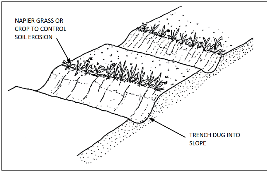
Figure 7-1: Bench Terraces (slope < 55%)
Bench terraces can be developed from grass strips, which in their turn can start as either unploughed strips, grass planted in one or two rows (e.g. Napier grass) or trash lines laid along the contours. Figure 7-2 shows how manual labour and erosion together can develop a bench terrace from a grass strip.
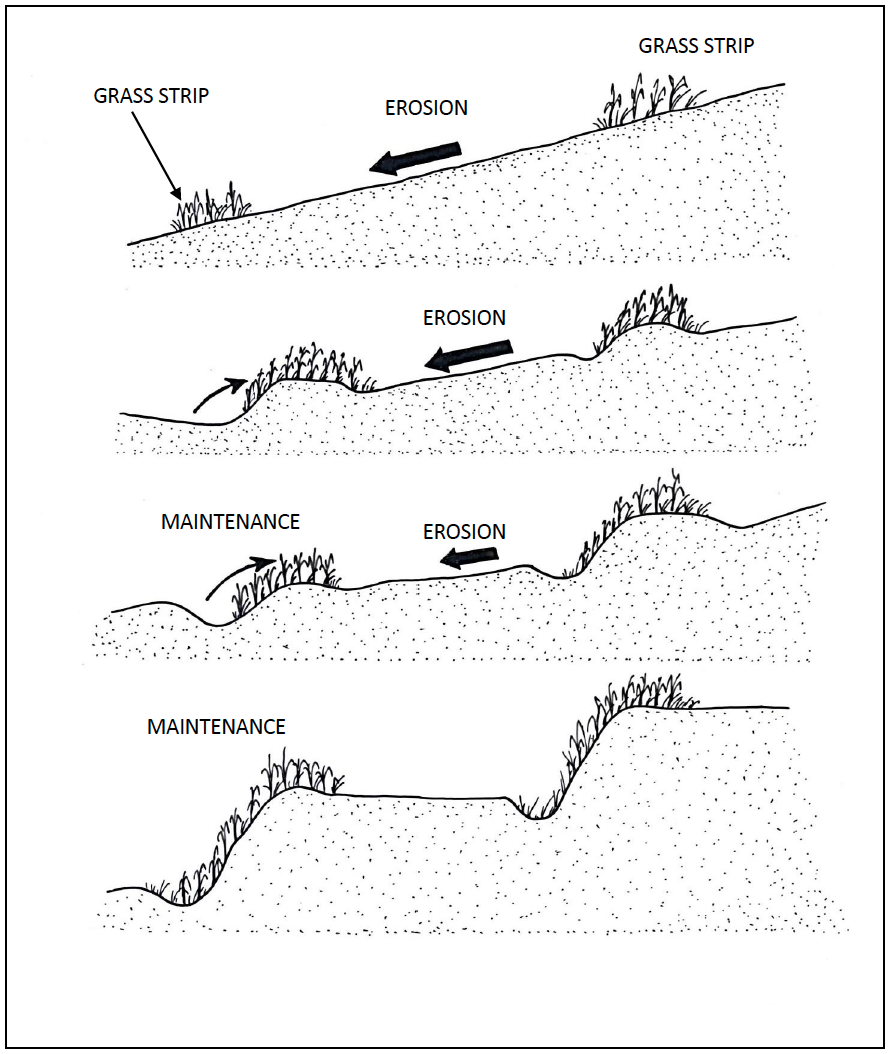
Figure 7-2: Development of Bench terraces from Grass Strips
To hasten the development of a bench terrace, or on steep slopes, the so called Fanya Juu method can be used (See Figure 7-3). A channel is dug and the soil thrown uphill to form an embankment (ridge). Grass should be planted on the ridge to protect it. Part of the channel should be maintained as a storm water drain. In dry areas an infiltration ditch may be better except on steep slopes or unstable soils. On rocky ground, stones can be collected and set in a small ditch to act as a barrier.
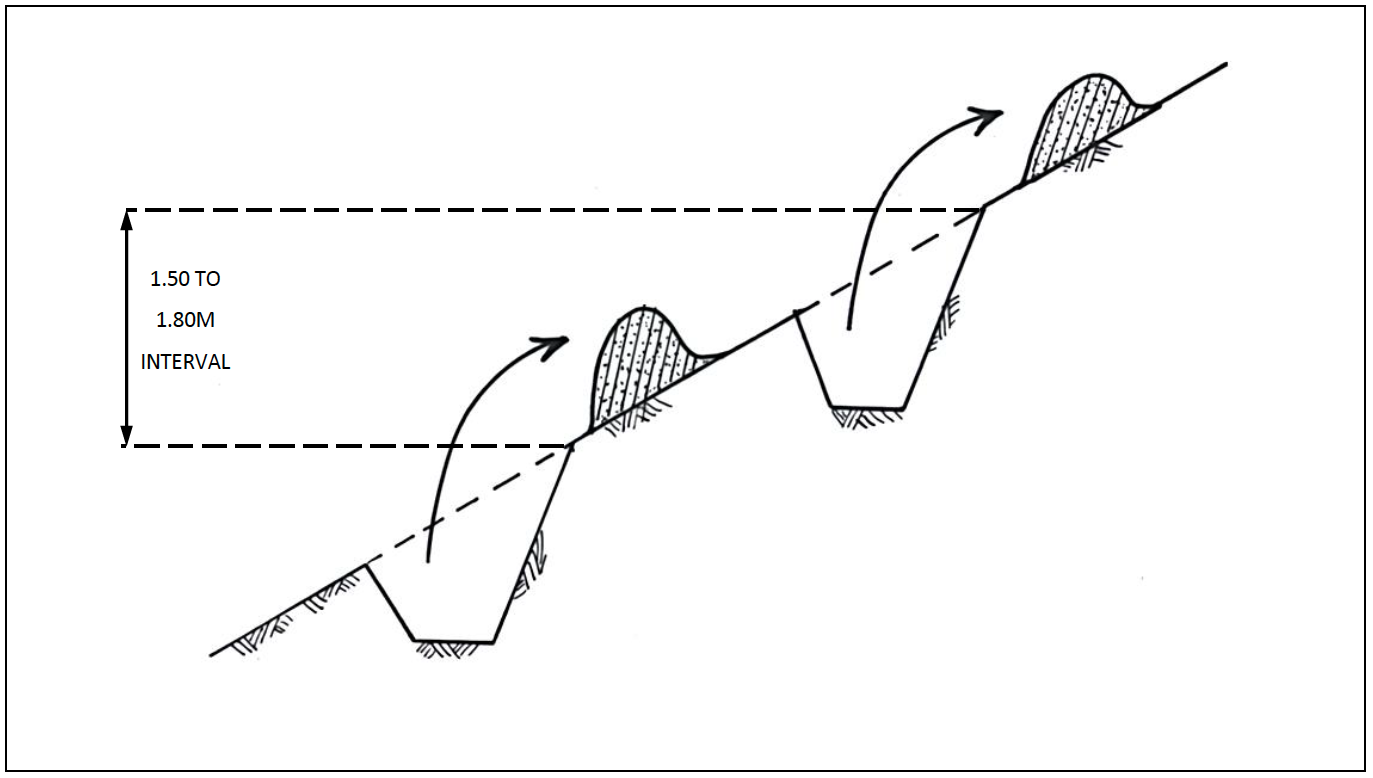
Figure 7-3: "Fanya Juu" Terracing
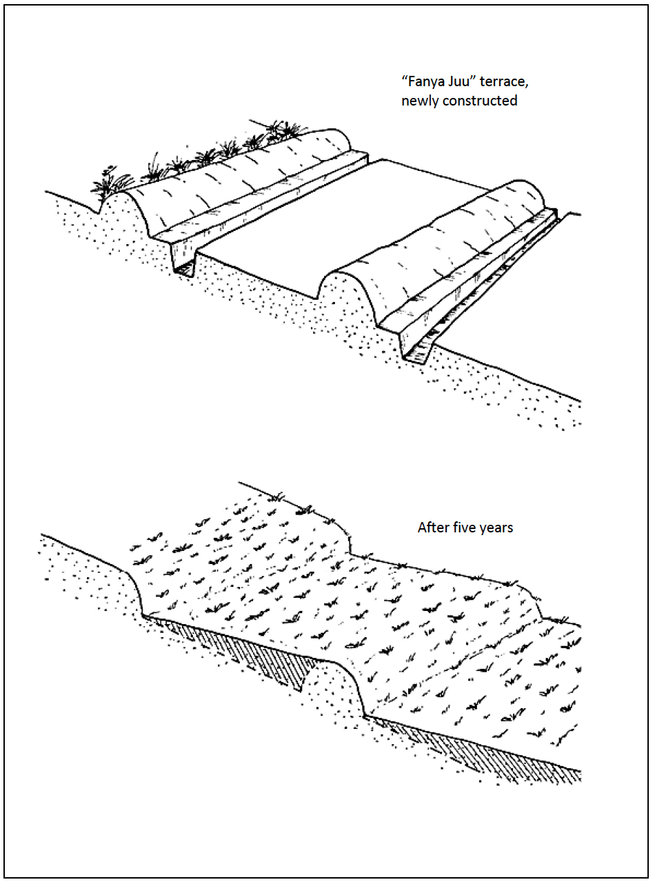
Figure 7-4: Progression of a Fanya Juu Terrace
Modified bench terraces (see Figure 7-5) can be used on steep and very steep slopes, for the planting of trees.
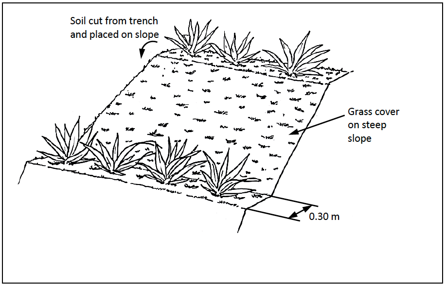
Figure 7-5: Modified Bench Terraces (35% < slope < 55%)
Mechanised terracing can be used on slopes not exceeding 12%. Two types are used in Kenya: the channel type and the ridge type. (See Figure 7-6) They will basically develop into bench terraces, as the channel fills up with sediment.
Dimensioning of Terraces: It is preferable to use a constant vertical interval of between 1.5 and 1.8 m (corresponding to the eye height of a person) in setting out terraces. For the variations which in some cases are applicable reference is made to Thomas D.B. ((ed.) 1997).
Terraces should not be longer than about 400m. However, if it is difficult to find a natural waterway or a non-erodible area to discharge water within that distance, it might be cheaper to make the terraces longer than to construct an artificial discharge channel.
Terraces should usually be sloped. Table 7-2 gives an indication of slopes recommended for terraces and cut-off drains. In dry areas it is preferable to make the terraces level to retain as much water as possible in-situ.
Table 7-2: Recommended Slopes for Terraces and Cut-off Drains
Soil Type Recommended Slope (%) Erosion resistant (Clay) 1 Normal 0.5 Erodible (silty, sandy) 0.25 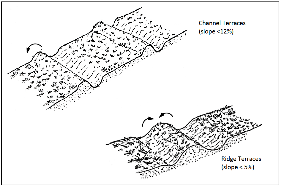
Figure 7-6: Mechanised Terracing
7.4.4 Use of Artificial Waterways and Cut-Off Drains
-
Cut-off Drains/diversion ditches: Preventing water from flowing down terraced slopes, or diverting large quantities of water from entering farms can be achieved by using cut-off drains. However, cut-off drains should only be used where there is evidence of large flows of water which cannot be stopped through normal terracing. Cut-off drains should be constructed only after terracing has been carried out.
An essential aspect when planning the construction of a cut-off drain is the location of the outlet point. Cut-off drains should not be constructed in locations where the water cannot be discharged safely.
Cut-off drains should further only be constructed where a sufficient level of community involvement can be obtained to guarantee regular maintenance (removal of silt from the channel etc.) by the farmers.
Approximate dimensions of manually constructed cut-off drains are shown in Figure 7-7. In Fanya Juu terracing, the top terrace should be constructed as a cut-off drain, with the soil being thrown down the slope so that the channel can carry as much water as possible. Mechanically dug cut-off drains have often a V-shaped cross-section and are somewhat larger than shown on Figure 7-7. Recommended slopes for cut-off drains are given in Table 7-2. Cut-off drains should not be longer than approximately 400m.
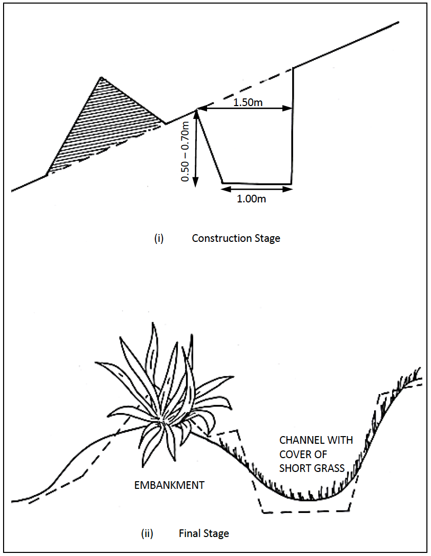
Figure 7-7: Cross Section of Cut-Off Drain
-
Artificial Waterways: The water from cut-off drains as well as from terraces should be discharged into natural watercourses (rivers) or onto non-erodible areas, such as rocky ground or permanent pasture with a good grass-cover. If such an outlet point cannot be found within a reasonable distance, an artificial waterway will have to be constructed to take the water down the slope (see Figure 7-8).
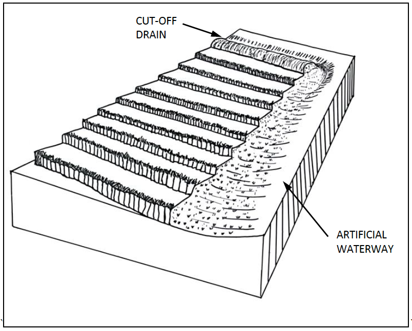
Figure 7-8: Discharging runoff along an artifical waterway
Such artificial waterways should be wide (at least 1.50 m), shallow (0.30 m deep) and should have a short grass cover in order to minimize erosion.
An appropriate method of constructing these waterways is shown on Figure 7-9. For further details of dimensions and recommended slopes, reference is made to Thomas D.B. ((ed.) 1997).
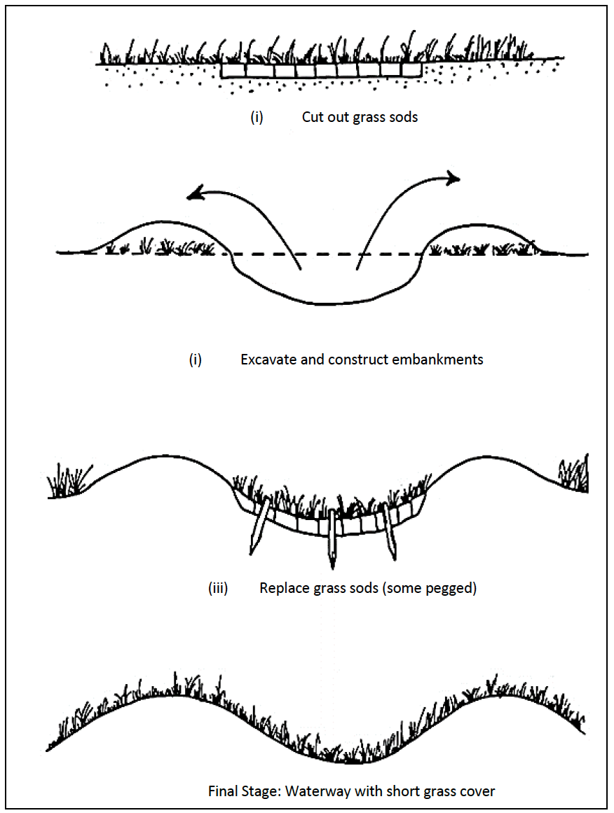
Figure 7-9: Construction of an Artificial Waterway
Artificial waterways and cut-off drains should not be constructed if proper maintenance is not guaranteed. Non maintained cut-off drains and artificial waterways will easily deteriorate into gullies, and are as such worse than nothing.
7.5 Control of Gully Erosion
When rills have increased in size so that they cannot be levelled out by ploughing, they are called gullies. The mechanics of gully development are explained in Figure 7-10. First, at the head of the gully, erosion will cut back into the slope [(i)]. Thereafter, the flow over the floor of the gully will deepen it, until solid rock is reached [(ii)]. The gully will further be widened by soil which is rendered unstable by the deepening of the gully, eventually sliding into the gully [(iii)]. A V-shaped gully is indicative of a gully that is still forming and active erosion is taking place. A U-shaped gully indicates that the erosion surface is along the sides of the gully, rather than the floor or headwall.
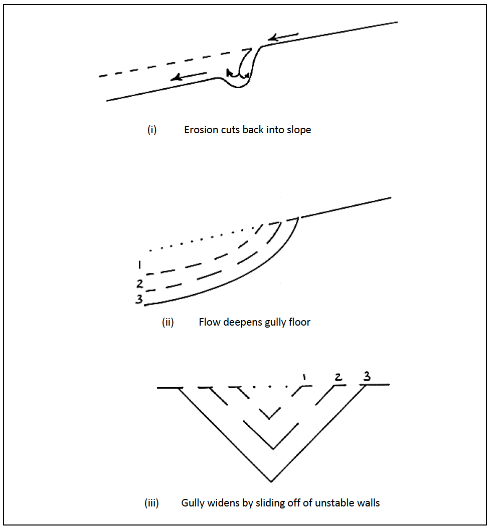
Figure 7-10: Mechanism of Gully Development
In its early stages, it is usually not difficult to stop gully erosion. Unfortunately gullies are usually left to develop until they cannot be returned to cultivated land. Small gullies (up to 0.50 m deep) can be filled with soil, brushwood, hay etc. Restoration of large gullies requires a great deal of time, effort and money. In terms of simple economics, the repair of gullies is seldom justified in semi-arid regions with soils of low agricultural value. However, an economic analysis should be undertaken before deciding whether the works are justified or not.
The main measures to contain gully erosion can be summarized as follows:
- Diverting the water from the head of the gully by means of a cut-off drain, or a ridge of soil. If this is possible, no other measures are needed in the gully itself.
- If diversion is not possible, then the velocity of the water needs to be reduced by means of scour checks and check dams. The head and floor of the gully need to be protected with erosion resistant materials. The type of measures used will differ according to the shape of the gully, and the availability of construction materials.
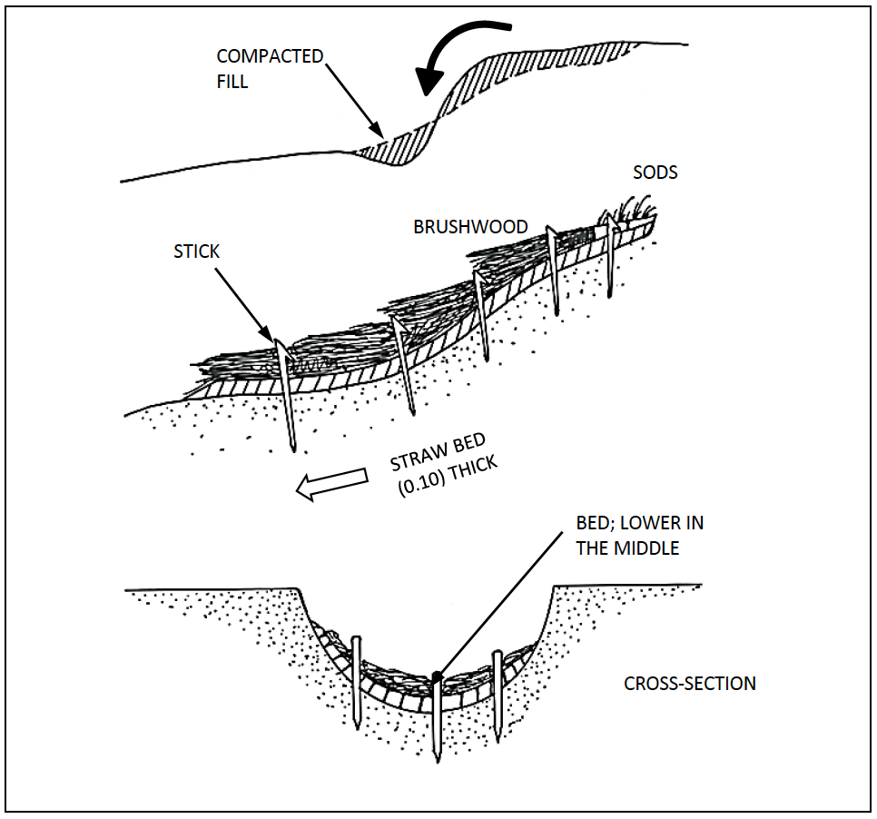
Figure 7-11: Gully Head Protection Using Wood
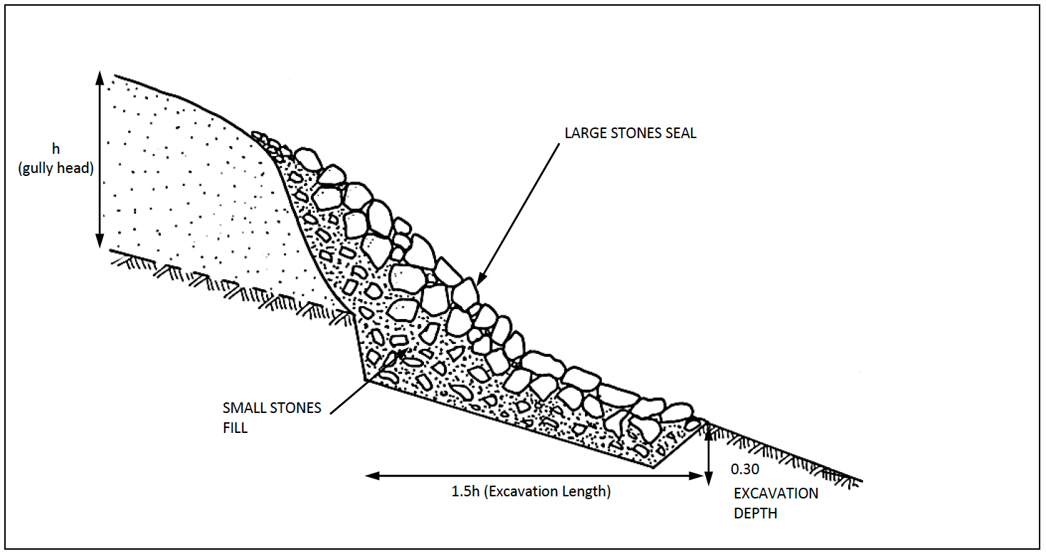
Figure 7-12: Gully Head Protection Using Stones (h<1m)
-
Head of gully: Figure 7-11 to Figure 7-13 show adequate protection measures in various cases. In case only small stones are available, gabions will be used. Note that care should be taken when developing gabions to arrange stones inside gabion box so that the galvanising on the wire is not damaged and that the stones are stable in the event that the wire rusts and breaks.
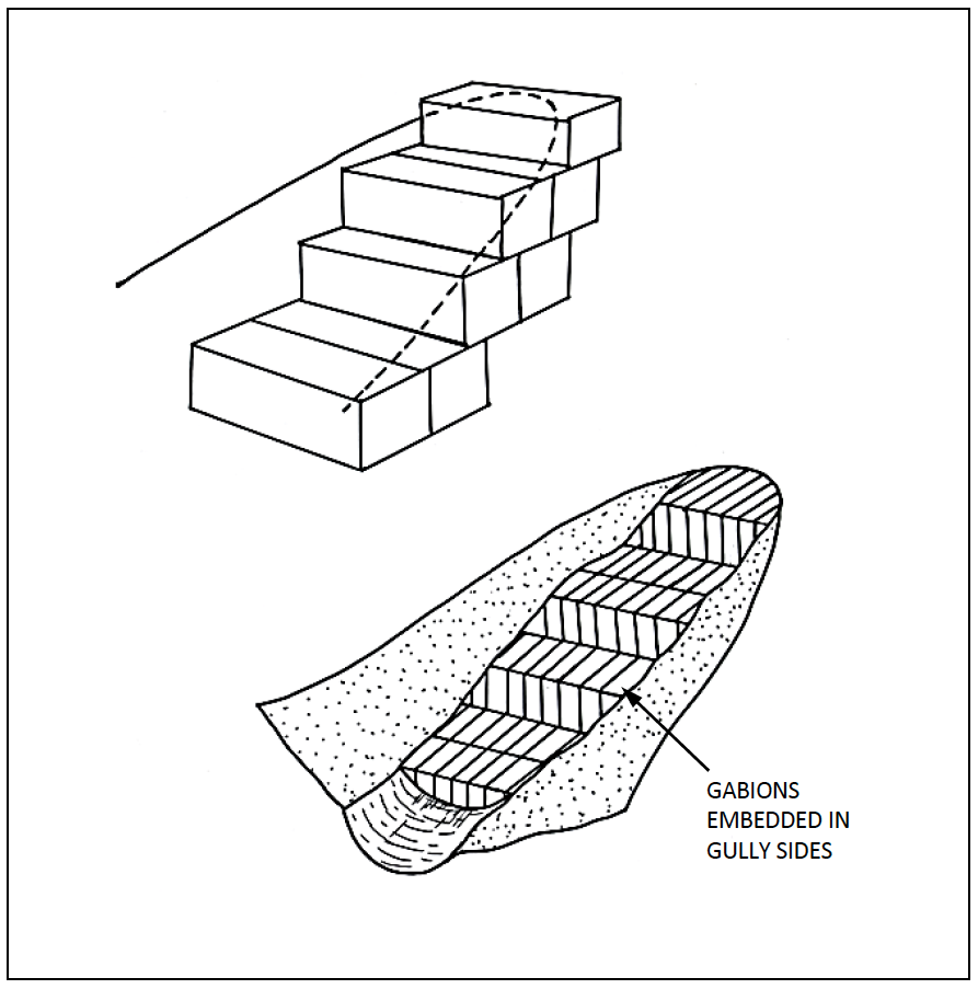
Figure 7-13: Gabion Gully Head Protection
-
Gully Floor: Figure 7-14 shows how stone thresholds can be used to protect the floor of wide and shallow gullies. In case of steep and V-shaped gullies, check dams made using large stones or gabions as shown on Figure 7-15 and Figure 7-16 respectively can be used. Check dams should be lower than one metre and they must not block the gully valley.
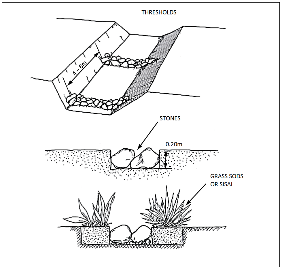
Figure 7-14: Stone and Grass Thresholds
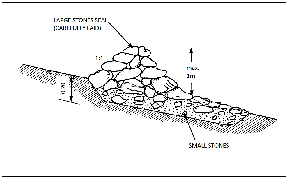
Figure 7-15: Cross Section of a Check Dam
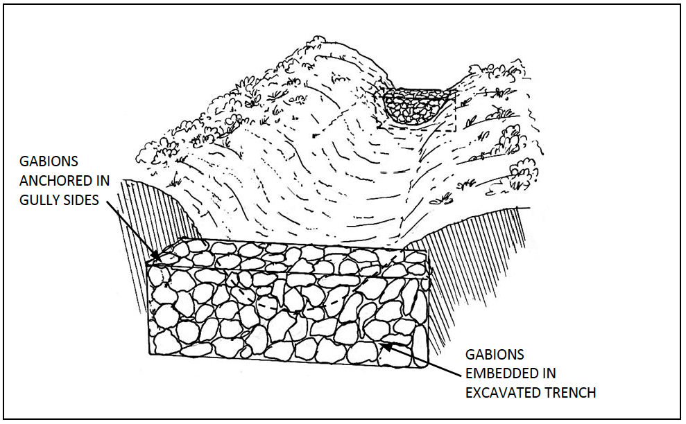
Figure 7-16: Gabion Check Dam
7.6 Protection of River-Banks
The quantity of sediment transported in a river depends largely on the rate of erosion of the catchment area. When sediment inflow into a river is reduced by the use of soil conservation methods in the catchment area, the river will tend to scour or cave its banks in order to regain its normal sediment load. Therefore, riverbank protection is necessary as part of a sediment control plan.
A river cannot erode above its highest water level (flood level). Erosion is most likely to occur in the stretches of the river where the water velocity is highest. In wide sections of the river (flood plains etc.) where low velocities occur, erosion protection measures are normally not required.
7.6.1 Riparian Area
Agricultural, environmental and water regulations specify the width of the riparian strip. In general it is a minimum of six metres, a maximum of 30 metres or otherwise half the width of the river (bank top to bank top) and is measured from the river bank edge. Riparian legislation addresses land use and not land ownership, as is frequently and mistakenly understood. The riparian legislation defines the width and which activities are not allowed within the riparian area, unless with government approval. The activities proscribed such as cultivation, development of permanent structures and latrines, grazing of livestock, etc., are aimed at ensuring proper ground cover and minimising the likelihood of human, agricultural or livestock pollution of the water body.
7.6.2 Riverbank Protection by Vegetation
Natural vegetation up to the flood level should be protected as much as possible. In cases where the natural vegetation has been removed by the streamflow, it should be replaced with permanent grass or trees.
Cultivated slopes above the flood level should be considered as ordinary slopes with regard to terracing (see Section 7.4.3)
7.6.3 Mechanical Riverbank Protection
In many cases vegetation alone will not provide sufficient protection against the scour of the water and mechanical protection will be required.
Gabions can be used to build stepped walls, while rip-rap (a cement grout can be brushed in if required) or Reno Mattresses are appropriate for protecting sloping banks.
Care must be taken to ensure that the intervention to protect the riverbank does not actually make the situation worse by disrupting the riverbanks. A “do no harm” approach should be taken and where mechanical measures cannot be done adequately to guarantee success, then alternatives of improving vegetation cover on the river banks should be considered.
7.7 Erosion Control on Grazing Land
7.7.1 Erosion on Grazing Land
Development of erosion follows a typical process. Through overgrazing and droughts bare spots will come into existence and increase in size. Perennial grasses are replaced by annual grasses and weeds. The bare soil is compacted by on-going trampling of cattle, thus increasing the run-off. Rain and rill erosion remove the topsoil. Gullies will start on slopes and develop by cutting back until the bedrock is reached, or alternatively up to the hillcrests. Later on the gullies will develop branches which will prevent normal cultivation and grazing.
7.7.2 Erosion Control Measures
Grazing control is the most important control measure on grazing land. Rotational grazing (including the closing of areas if required) and de-stocking where required are the most important components of grazing control.
For rehabilitation deep and loamy soils are best suited. Rehabilitation should only be attempted in areas with annual rainfall over 300 mm. Rehabilitation can start as follows:
- Closing an area, and thereby allowing natural grasses to establish a new cover. To increase infiltration contour ploughing can be carried out. A spacing of three metres between the ploughing furrows should be maintained on land with some weeds and grass, while a one metre spacing is suitable for completely denuded land.
- Closing and re-seeding, with suitable species of grasses after some land preparation. Usually scratch ploughing is needed. It is best to re-seed at the beginning of the rainy season. Perennial grasses should be used. As to recommended species, reference is made to Thomas D.B. (Eds. l997).
Finally, it must be emphasized that:
- Measures against erosion without grazing control are useless.
- Cut-off drains especially in sandy soils are useless without grazing control measures and establishment of grass cover around the gullies.
7.8 Control of Road Runoff
Nagle (1999) quoting sediment yield rates in Kenya by Dunne (1979) estimates that roads and trails may contribute 25 – 50% of total sediment yield, although they only constitute a small percentage of the land area (typically less than 2%). While these sediment yield estimates are based on basins with steep settled agricultural land, it is indicative of the scale of the problem which is generally given insufficient attention by road engineers and contractors and soil conservation practitioners. Essentially the runoff from road servitude and surrounding areas, if not properly controlled, can cause extensive damage to the roadway and to adjacent property.
This calls for the provision of (1) appropriate drainage structures on the road to reduce the concentration of and manage the runoff and (2) suitable erosion control structures to protect adjacent land where the road runoff is discharged.
Eriksson and Kidanu (2010) address this issue comprehensively in the Guidelines for Prevention and Control of Soil Erosion in Road Works. A brief summary of the key points is presented herein.
7.8.1 Genesis of the Problem
Roads and tracks are made by removing the natural vegetation and providing a compacted surface for traffic. The road surface itself is therefore designed to be impermeable and will generate runoff. The roadway is either elevated above or cut into the natural ground level and so either way, will intercept any flow paths that it crosses, thereby concentrating runoff into the roadway.
While the government road authorities are clearly responsible for the drainage within the road reserve, there is less clarity on who is responsible once the runoff leaves the road reserve. This ambiguity results in land owners having to deal with runoff problems, not of their making, that they perhaps do not have sufficient technical and/or financial resources to deal with or preventing road drainage onto their land thereby threatening the road.
7.8.2 Controlling Upland Runoff
The first step is to reduce the amount of runoff being collected by the roads through better soil and water conservation in the upland areas of the catchment, whether they are forested, agricultural or grazing lands. This may also include harvesting rainwater from roofs and paved areas into tanks and short-term retention ponds. In addition, cut-off drains can be constructed to intercept the runoff prior to reaching the road for safe disposal. The size, slope and surface cover of the drains need to be carefully designed to avoid creating a gully. See “Guidelines for Prevention and Control of Soil Erosion in Road Works” (Eriksson & Kidanu, August 2010) for details on sizing artificial waterways.
Insufficient attention to controlling upland runoff can result in more complicated and expensive structures in the road or lower catchment.
7.8.3 Road drainage
Road drainage generally includes the following components:
- Side drains. Reduction of erosion in the side drains along the edge of the road is achieved by controlling the water velocity. This can be accomplished by forming and lining the drain, and installing scour checks, check dams and/or drop structures.
- Mitre drains. These are used to discharge accumulated runoff in the side drains into adjacent land. This is possible where the roadway is above or close to the natural ground level and impossible where the roadway cuts through an embankment. The interval of mitre drains can be as frequent as 20 metres in high rainfall, steeply sloped land. Mitre drains need to be cut at a slope of ≈5% and kept clear of sediments.
- Culverts. This are constructed with suitable inlet and outlet boxes to pass runoff under the roadway from where it either discharges into the side drain on the lower side of the road or where it is directed away from the roadway to the river or natural water course. This may require a purposefully designed water way.
- Bridges. Bridges are required to enable the roadway to pass above a natural water course. If the bridge does not have sufficient capacity to safely pass floods, then scouring of bridge abutments can occur; flood waters can look for alternative routes thereby creating the likelihood of erosion in other areas.
-
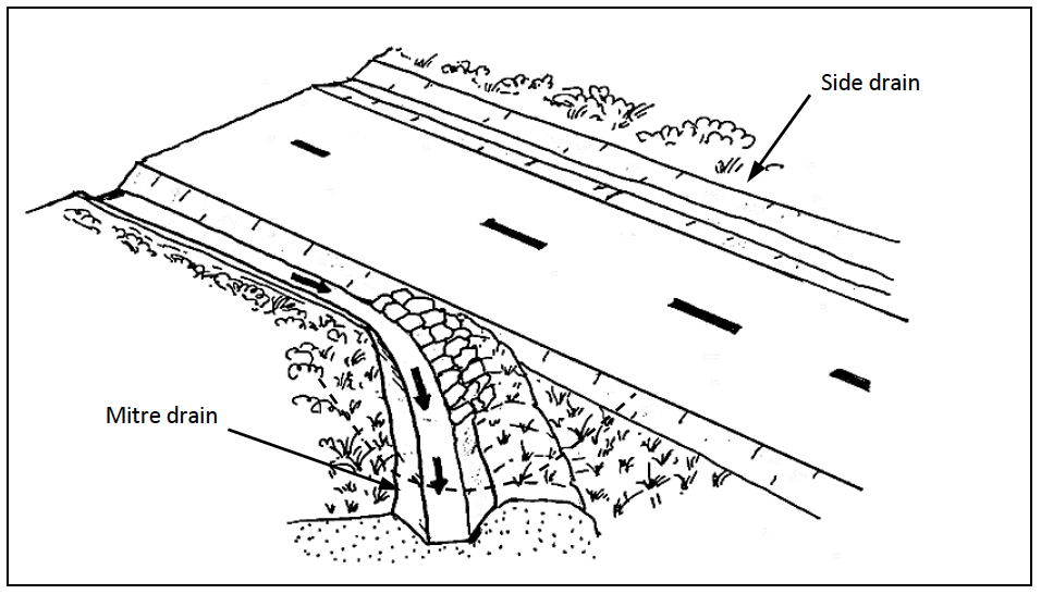
Figure 7-17: Example of a Mitre Drain and Side Drain
All of the road drainage structures require maintenance to remove sediment, and woody vegetation, frequent inspection (i.e. after each rainy season) and remedial work undertaken to arrest any scouring, gully formation, or degradation of the structures.
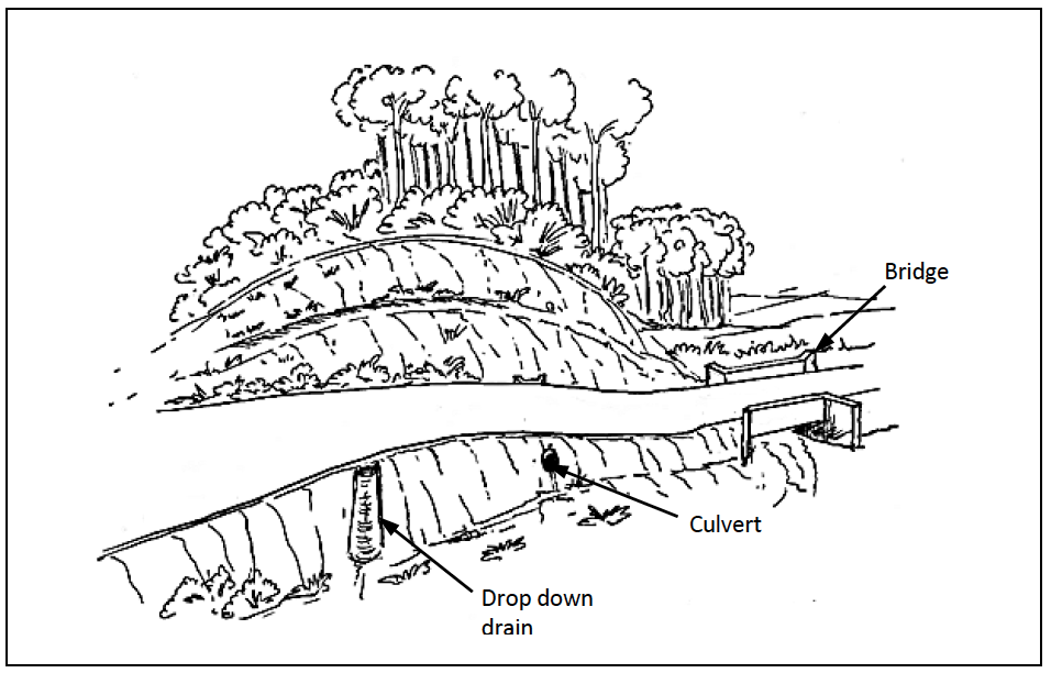
Figure 7-18: Illustration of Different Types of Road Drainage
7.8.4 Controlling Runoff in the Lower Catchment
The runoff that has been discharged from the roadway, through mitre drains or from culverts, should either be:
- dispersed to soak into the adjacent ground;
- channelled to an infiltration ditch;
- channelled in a purpose built waterway to convey the water safely to the natural water course;
- channelled to a water conservation structure (e.g. pan).
This frequently requires the design of an artificial waterway (e.g. vegetated or stone pitched channel) or outfall channel.
7.9 Stabilisation of Road Embankments
Where a road cuts through an embankment or is placed along the side of a hill, there is typically a steep bare slope on both sides of the road, either rising or falling away from the roadway. The road embankments are prone to erosion and should be stabilised through grassing on and above the slope or through the use of Reno Mats.
7.10 Control of Spillway Discharge
Although most of this chapter has concentrated on erosion control above the proposed storage structure, it is also necessary to consider the downstream erosion risks that the storage structure may generate. Spillways should be designed to minimize erosion and the use of gabions, concrete sills or other energy dissipating structures should be considered to ensure that the storage structure itself does not contribute to erosion within the catchment.
7.11 Financing Conservation Activities
Proper catchment management is essential to the performance and sustainability of water retention structures within the catchment. However, the activities involved are often time consuming and expensive.
Several options are currently available for financing catchment conservation activities. As earlier mentioned, the Water Services Trust Fund offers financial support to WRUAs for the implementation of their sub-catchment management plans.
Other private conservation organizations can also be approached to fund similar activities. Private companies are also a potential source of funding. Proposals can also be developed to incorporate catchment conservation into their corporate social responsibility (CSR) activities.
As many of the activities rely heavily on local labour, prices should be adjusted to reflect current labour costs.
8 Hydrological And Sediment Analysis
This section presents the hydrological analysis required to support the design of a small dam, pan and other water storage structures. This chapter provides various methods to address the following issues with respect to a proposed project:
- Is there sufficient inflow?
- How much storage capacity is required?
- What are the peak design flows that need to be passed safely by the structure?
- What are the design flows for diversion or ancillary structures?
- What are the environmental flow requirements?
8.1 Introduction
The level of hydrological analysis required will depend on the size and nature of the structure being proposed. It is helpful to know what the design criteria are for the proposed structure as this will direct the outputs required from the hydrological analysis.
8.2 The Hydrological Cycle
The hydrological cycle is a conceptual model that describes the continuous cycle of storage and movement of water on, above and below the Earth’s surface.
Understanding the hydrological cycle provides insights into the processes involved in the movement of the earth’s waters, and this knowledge can be utilised in planning, engineering and water resource management.
Figure 8-1 below illustrates the various stages of the hydrological cycle. The hydrologist’s primary focus, in respect of this manual, is on the run-off component, as this provides an indication of the water available for storage.
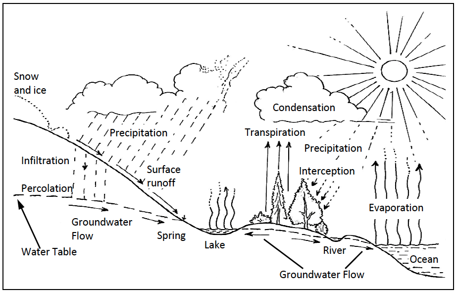
Figure 8-1: The Hydrological Cycle
8.3 Hydrological Design Criteria
Reference should be made to Chapter 2 to determine the Class of Dam based on the Water Resources Management Rules (2007) which also provide minimum design standards for storage structures of different classes as shown in Table 8-1. More conservative design criteria have been recommended herein to allow for various factors including:
- Catchment conditions are changing rapidly in some areas due to rapid urbanisation;
- Climate change predictions indicate rainfall of higher intensity;
- Risks associated with future settlement downstream of the structure.
Table 8-1: Return Period Criteria for Design Purposes
| Class of Dam | Minimum Return Period for Design of Spillway (WRM Rules 2007) | Recommended Minimum Return Period for Design of Spillway | Recommended Minimum Return Period for Design of Diversion Works, if required |
|---|---|---|---|
| A (Low Risk) | 1 in 50 years | 1 in 100 years | 1 in 5 years |
| B (Medium Risk) | 1 in 100 years | 1 in 100 – 500 years | 1 in 10 years |
| C (High Risk) | 1 in 500 years | 1 in 1000 years | 1 in 15 years |
(Source: WRM Rules 2007)
Reference should be made to ICOLD guidelines for Class C dams. The Probable Maximum Flood (PMF), or the most severe flood event reasonably possible in the catchment should be considered during spillway design for Class C dams, but is generally not a requirement for Class A or B dams. However, a critical review of the potential downstream impacts associated with a dam failure should inform the final selection of the hydrological design criteria, even for Class A and B dams.
The design criteria for diversion works requires further discussion. The construction of diversion works can add a significant cost to the overall project cost. However, failure to provide adequate facilities for diversion of flow can impede construction or damage works already constructed.
One way to mitigate the cost of the diversion works is to schedule construction during the dry season or low flow period. In this case diversion works may not be necessary or can be reduced to accommodate minor flood events. In this case, the hydrologist may use the rainfall and flow data strictly from the expected construction period, using the criteria specified in Table 8-1 to determine the required capacity for the diversion works. It should be noted that, if the construction activities do not follow the stipulated construction plan, then any design based on assumptions regarding the construction schedule, will need to be reviewed and appropriate steps taken.
For storage structures other than dams for which design criteria are not specified in the WRM Rules (2007), the hydrological design criteria should be based on the following factors:
- The inflow to the structure should be of sufficient quantity, quality and reliability to justify the investment in the structure;
- The structure should be able to pass an extreme inflow event of a specified return period without damaging the structure or downstream environments. The return period to be used will be a function of the scale of investment and the risk posed to downstream environments. Therefore the return period for a sand dam or sub-surface dam may be a 1 in 50 year event although for an offline pan (not on a water course) a 1 in 10 year event may be appropriate.
8.4 Data Requirements
The quality of the hydrological analysis will depend in part on the availability of reliable data. The data user should expect to prove the reliability and consistency of any data sets he/she has obtained.
In general, the longer the record the better as the data set will reflect more extreme events and provide more confidence in the results. The computing power now commonly available means that data sets containing multiple records of more than 50 years can be analysed with ease. Table 8-2 provides a general listing of the data requirements and possible sources.
Table 8-2: Hydrological and Meteorological Data Requirements
| Data Type | Detail | Comments |
|---|---|---|
| Rainfall | Location of rainfall stations within or neighbouring the catchment area and length of the record | Obtained from WRMA or KMS This facilitates the identification of which data sets should be pursued. |
| Daily (24 hour ) rainfall | Number of stations will depend on catchment size but at least 3 to 4 stations within or neighbouring the catchment area. Obtained from WRMA, KMS or from the station itself. Internet based rainfall records are also available, but check reliability and accuracy. | |
| Mean monthly rainfall | Derived from daily data or obtained from KMS. | |
| Mean annual rainfall | Derived from daily data or obtained from KMS. | |
| Annual 24 hour maximum | Derived from daily data or obtained from KMS. | |
| Rainfall-duration-frequency | Rainfall Frequency Atlas of Kenya (MoWD, 1978) NWMP (1992), NWMP 2030 or from Automatic Weather Stations (KMS, Syngenta, WRMA). | |
| Evaporation | Mean monthly open water evaporation | Obtained from Chapter 3 this Manual or KMS or the FAO CropWat website. |
| Discharge | Location, reference number of river gauging stations and duration of the record | This facilitates the identification of which data sets should be pursued. |
| Approved discharge rating equation(s) for selected RGS | WRMA. | |
| Daily discharge data | WRMA. | |
| Catchment | Catchment boundaries | Derived from topographical map (obtained from Survey of Kenya) or calculated from a Digital Elevation Model (DEM). WRMA. |
| Contours | Derived from topographical map or calculated from a Digital Elevation Model (DEM). | |
| River drainage network | WRMA. | |
| Land use map | FAO/Africover website. | |
| Vegetation cover | FAO/Africover website. | |
| Soil map | FAO/Africover website. | |
| Geological maps & Reports | Department of Mines & Geology. | |
| Cadastral maps | Provides information on land ownership. Survey of Kenya, Ministry of Lands. | |
| Seismic maps | Department of Mines & Geology. | |
| Water Resource Allocations | Existing authorisations within the catchment | WRMA. |
8.5 Data Availability and Reliability
It is generally considered good practice for a hydrologist or engineer who is using hydro-meteorological data to verify the location and on-site conditions for the data that is being used. This eliminates basic problems regarding the datasets.
The time-series data availability should be plotted as shown in Figure 8-2. The data availability chart provides a visual presentation of the available data. The length and consistency of the record can be seen and compared. This helps in the selection of the data for further analysis. Further investigation of the data is required to determine data gaps and to assess the usefulness of the dataset.
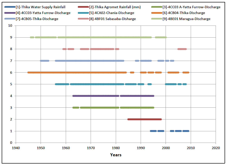
Figure 8-2: Sample Data Availability Chart
No analysis of any data sets should be undertaken until the data has been cleaned and there is confidence that the data provides an accurate record of the measured parameter.
The quickest method to check the reliability of the data is to use double mass plots as set out below:
- Select two preferred rainfall stations;
- Eliminate from both records any day in which either of the stations has a missing value;
- Plot the resultant cumulative daily rainfall of each station on the X and Y axis;
- Examine the plot. If the relationship between X and Y is reasonably constant (See Figure 8-3) the graph should plot as a straight line of uniform gradient. Change of gradients and undulations reflect an inconsistent relationship and may be explained by inaccurate data in one or both records;
- Identify the general gradient and then eliminate inconsistent periods from both data sets;
- Repeat the exercise with different combinations of rainfall stations, paying close attention to which combination provides the longest record of consistent data.
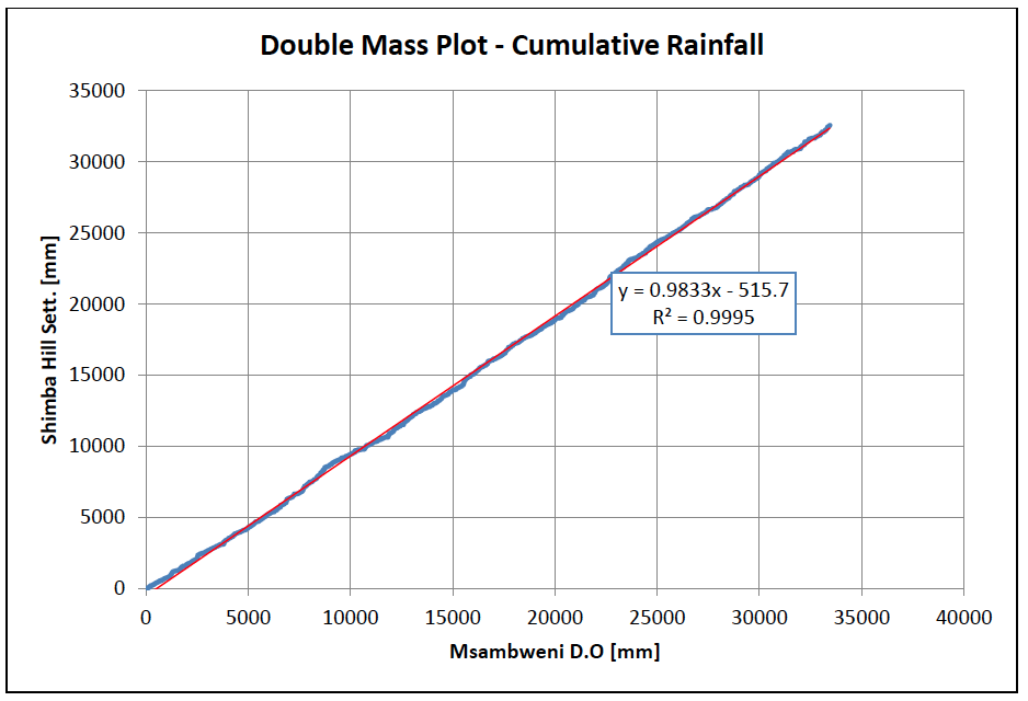
Figure 8-3: Sample of a Double Mass Plot of Two Reliable Rainfall Stations
Once at least one good quality rainfall record has been identified, the double mass methodology can be applied between the good rainfall record and the discharge time series. Again, periods of inconsistent data should be flagged in the discharge time series and removed from the data analysis. The result should be a line of fairly uniform gradient. Note that some variability can be expected due to natural variations in catchment conditions, rainfall location and intensity etc.
In the event that a non-uniform line is obtained, further investigations should be conducted on the discharge data. This will involve the following steps:
- Obtain water level time series from WRMA and review the general pattern, looking for anomalies, trends, extreme values outside the realm of possibility, etc.;
- Review the gauging data against the approved discharge rating equation to establish whether the rating equation matches the gauging data.
The final result of the consistency check should be a set of rainfall and discharge data for which there is confidence in its integrity.
8.6 Rainfall Analysis
Rainfall analysis should be conducted to provide three simple outputs:
- Mean monthly rainfall. This is used to determine the longest and driest period and is used to estimate storage requirements and to select the best time to schedule construction activities. Median monthly rainfall, being less influenced by extremes, can also be used;
- A time series of mean annual rainfall and the long term mean value;
- Rainfall frequency.
It should be noted that the location of the rainfall station(s) should preferably be within the catchment area and upstream of the site under investigation. Appendix A provides a map of mean annual rainfall for the country.
8.6.1 Rainfall Frequency Analysis
Rainfall frequency analysis is an important component in the estimation of peak flows for specific return periods, especially where there are no stream flow records. A basic assumption is made that the return period for a storm corresponds to the return period for flows.
Furthermore, the duration of the storm should correspond to the time of concentration of the catchment (tc). (See Section 8.10.2 for determination of time of concentration).
The Rainfall Frequency Atlas of Kenya (Ministry of Water Development, 1978) provides rainfall-duration-frequency (RDF) maps for the whole of Kenya for different combinations of storm duration and return periods as shown in Table 8-3. These maps are essential where the time of concentration is significantly less than 24 hours, which is the case for small catchments.
Table 8-3: Storm Duration-Frequency Combinations
| Return Period (Years) | |||||
|---|---|---|---|---|---|
| Duration | 5 | 10 | 25 | 50 | 100 |
| 10 min | ✔ | ✔ | ✔ | ✔ | ✔ |
| 30 min | ✔ | ✔ | ✔ | ✔ | ✔ |
| 1 hr | ✔ | ✔ | ✔ | ✔ | ✔ |
| 2 hr | ✔ | ✔ | ✔ | ✔ | ✔ |
| 3 hr | ✔ | ✔ | ✔ | ✔ | ✔ |
| 6 hr | ✔ | ✔ | ✔ | ✔ | ✔ |
| 12 hr | ✔ | ✔ | ✔ | ✔ | ✔ |
| 24 hr | ✔ | ✔ | ✔ | ✔ | ✔ |
(Source: Rainfall Frequency Atlas of Kenya, 1978)
For larger catchments, the 24 hour rainfall frequency can be established based on the annual maximum 24 hour rainfall series. This time series can be analysed using extreme event distributions to obtain the estimated 24 hour rainfall for different return periods. An open source statistical software (e.g. Easyfit) can be used to fit different probability distributions to the annual maxima data series. Care should be taken to select probability distributions appropriate for rainfall analysis e.g.:
- Gumbel – EV Type 1;
- Frechet - EV Type II;
- Weibul - EV Type III;
- Log-Pearson Type III;
- Log Normal Distribution;
- Wakeby Distribution.
8.6.2 Catchment Rainfall
Rainfall is unlikely to occur equally over a catchment, especially for larger catchments. A single rainfall record has therefore to be adjusted by an area reduction factor (ARF) which is dependent on the size of the catchment as shown in Figure 8-6 and Figure B7.7 in NWMP 1992.
In the event that a number of reliable rainfall records are available for a particular catchment area, then a better estimate of the rainfall over the catchment on a storm, seasonal, or annual basis, can be made by using an area weighting factor as determined by the isohyetal, Thiesen polygon or a distance/gridded method.
8.7 Climate Analysis
The climate analysis is focused on mean monthly open water surface evaporation which is needed to estimate monthly evaporation losses from the dam or pan. See Section 3.3.10 for further details. A map of annual evapotranspiration is also provided in Appendix A.
8.8 Inflow Estimation
The aim is to obtain a fair estimate of the inflow to the storage structure. The method of estimation of the inflow to a reservoir will depend on the available data. A number of methods are set out below.
8.8.1 Estimation of Inflow without Discharge Data
Rough Estimate for Roof and Small Runoff Catchments (<5ha)
Monthly estimates of runoff volume from roof areas and small catchments (i.e. less than 5 ha) can be made using Equation 8-1.
Equation 8-1: $V_m = \frac{C.A.R_m}{1000}$
Where:
$V_m$ = runoff volume in month m [$m^3$]
C = runoff coefficient (Table 8-4)
A = catchment area[$m^2$]
$R_m$ = rainfall in month m [mm]
Table 8-4: Runoff Coefficients
Surface Type Runoff Coefficient (%) Roof tiles, corrugated sheets, plastic sheets, concreted bitumen 80 Brick pavement 60 Compacted soil 50 Uncovered surface, flat terrain 30 Uncovered surface, slope 0 – 5% 40 Uncovered surface, slope 5 – 10% 50 Uncovered surface, slope >1% > 50 Rough Estimate for Small Catchments (<10 Km$^2$)
Monthly and annual estimates of runoff are generally estimated to be between 10 – 20% of rainfall for the ASALs. Estimates of the runoff factor can be made from empirical data as shown in Table 8-5 for different catchments in East Africa or from values presented in NWMP 1992.
Table 8-5: Rainfall-Runoff Parameters for Small Catchments in Kenya
Catchments Area ($km^2$) Avg. Annual Rainfall (mm) Elevation range (masl) Predominant Land use Predominant Soil Type Annual Streamflow as % of rainfall Runoff Coefficient K for daily rainfall Threshold T for daily rainfall (mm) Laikipia Mukogodo 2.21 335 1770-1890 Grass-bushland Red clay loam 11 27.8 6.38 Ngenia 1.07 657 2110-2220 Small scale farming Red clays 9.1 22.3 7.94 Sirima 3.59 791 1940-2070 Small scale farming/ Black clays 2.6 10.7 11.9 bushland Kericho IJC13 Sambret 7.02 2026 2000-2800 tea Organic loams 37.8 IJC14 Lagan 5.44 2129 indigenous forest Organic loams 34.8 Mbeya A 0.2 1658 smallholder Organic loams 39.9 C 0.163 1924 indigenous forest Organic loams 28.1 Kimakia 10 C 0.65 2325 2000 – 3000
2440Bamboo Organic loams 45.6 11 A 0.36 1997 Pines Organic loams 41.6 17 (Makiama) 0.37 2062 Grass Organic loams 48.9 Atumatak 734 A 0.811 734 1345-1460 Grass/bush Shallow, sandy 7.8 – 14.4 B 759 Bush cleared, fenced 6.9 – 15.6 Multi-parameter Rainfall Runoff Models
There is a wide variety of rainfall runoff models from simple empirical models to complicated multi-parameter models that attempt to simulate hydrological processes. The decision to use multi-parameter models (such as NAM, SWAT, etc) should be made by experienced hydrologists. The use of complicated multi-parameter models requires rainfall and discharge data to calibrate and validate the model and can be data intensive.
8.8.2 Estimation of Inflow with Discharge Data
It is preferable to use discharge data from a reliable river gauging station near the proposed site. It is preferable to use naturalised flow data, although this is generally less significant for flood flow analysis and more significant for low flow analysis and inflow estimation. If the observed flow record is considered to be heavily influenced by abstractions, then use of historical data (i.e. prior to 1985) may reduce the influence of abstractions on the discharge data. The development of naturalised discharge time series would require an accurate time series of abstraction data for all the abstraction points in the catchment under investigation. However, historical discharge data may not adequately reflect current catchment conditions and catchment hydrological response. The hydrologist will need to make a value judgement regarding the most appropriate data to use for analysis.
Reliable discharge data from the study catchment or a similar catchment can be used to establish a discharge time series for the dam/reservoir site. It is reasonable to assume that the hydrological behaviour of two catchments are similar if the topography, rainfall, vegetation, soils, land use type and size are similar. Adjustments can be made for differences in size and rainfall using Equation 8-2.
Equation 8-2: $Q_A = \frac{P_A}{P_B} \times \frac{AREA_A}{AREA_B} \times Q_b$
Where:
$Q_A$ = discharge in catchment A (study catchment) [$m^3$/s]
$Q_B$ = discharge in catchment B [$m^3$/s] based on discharge data
$P_A$ = mean annual precipitation in catchment A (study catchment) [mm/yr]
$B_B$ = mean annual precipitation in catchment B [mm/yr]
$AREA_A$ = area of catchment A [$Km^2$]
$AREA_B$ = area of catchment B [$Km^2$]
This approach also applies if Catchment A and B are on the same watercourse and are in reasonable proximity (within 20 – 30 km).
8.9 Flow Frequency Analysis
Once a reliable discharge time series for the dam/reservoir site has been established, the probability of equalling or exceeding a particular flow can be established. The flow duration curve (FDC) presents a graphical description of the relationship between the frequency of exceedence and flow, as shown in Figure 8-4, with a spread sheet percentile function applied to the entire daily discharge time series.
Figure 8-4: Example of a Flow Duration Curve
The FDC provides the hydrological design values for the design of a self regulating weir, a water supply intake and the environmental flows (Reserve) (See Section 8.14 for Environmental Flows).
8.10 Flood Frequency Analysis
The design of spillways, diversion works and storm water channels require an estimation of the peak discharge for a given return period. Insufficient spillway capacity causing overtopping of the embankment with subsequent erosion of the downstream slope is a major cause of embankment failure (breaching) for small earth dams. This indicates the importance of establishing a conservation estimate of the inflow design flood (IDF).
8.10.1 Initial Estimate of Design Flood Flows
The Design Manual for Water Supply (Ministry of Water and Irrigation, 2005) provides estimates (Table 8-6) of the peak discharge rate for a 1 in 100 year return period based on the catchment area. The figures presented in Table 8-6 are typically used as estimates in the initial stages of a project and can be confirmed during the detailed design process with other methods.
Table 8-6: 100 Year Return Period Discharge
| Catchment Area ($km^2$) | $Q_{100}$($m^3$/s/$km^2$) |
|---|---|
| < 1 | 15 |
| 42009 | 42348 |
| 42149 | 42069 |
| 25 - 100 | 42065 |
| 100 - 1000 | 1 – 0.4 |
| > 1000 | < 0.3 |
8.10.2 Richard’s Method
An empirical method well suited for Kenyan conditions is given by Richards which uses rainfall data and catchment conditions. The method is based on an empirical formula to calculate the “time of concentration" ($T_c$) of the catchment. This is the time it takes for the rain fallen on the furthest point of the catchment to reach the river at the point where the peak flow is to be estimated. Richard’s method takes into account the rainfall pattern and intensity and the catchment characteristics determining its runoff: size, shape and slope, as well as soil and vegetation type (the latter two collated into a run-off factor $K_r$).
Table 8-7: Runoff Factors for Different Soil Types
| Catchment Soil Type | $K_r$ |
|---|---|
| Rocky and impermeable | 0.80 to 1.00 |
| Slightly permeable, bare | 0.60 to 0.80 |
| Slightly permeable, partly cultivated or covered with vegetation | 0.40 to 0.60 |
| Cultivated, absorbent soil | 0.30 to 0.40 |
| Sandy bare soil | 0.20 to 0.30 |
| Heavy forest | 0.10 to 0.20 |
The formula for calculating the time of concentration is shown in Equation 8-3 which is resolved iteratively for different values of $T_c$ until the equation balances.
Equation 8-3: $\frac{T_c^3}{(T_c + 1)} = \frac{C. L^2}{K_r . R . S . f(a)}$
Where:
$T_c$ = time of concentration [hours]
L = longest path of the catchment [km]
C = a coefficient, function of ($K_r$ . R) which can be obtained from Figure 8-5
$K_r$ = runoff factor, which can be obtained from Table 8-7
R = rainfall coefficient, where R = $\frac{(t+1)}{t}F$
t = selected storm duration [hours]. This should approximate the time of concentration ($T_c$).
F = total rainfall [mm] = intensity [mm/hr] x storm duration (t) [hours], for the selected storm duration and frequency. Intensity is obtained from the rainfall intensity maps in Appendix A or from the Rainfall Frequency Atlas of Kenya (KMS).
S = the average slope of the catchment.
f(a) = ratio of the average rainfall intensity (i) to the maximum rainfall intensity (I) over the catchment area, obtained from Figure 8-6.
a = the area of the catchment [$km^2$].
Once $T_c$ has been found, a revised estimate of the average rainfall intensity for the catchment can be established using Equation 8-4.
Figure 8-5: Coefficient C, Richard's Method
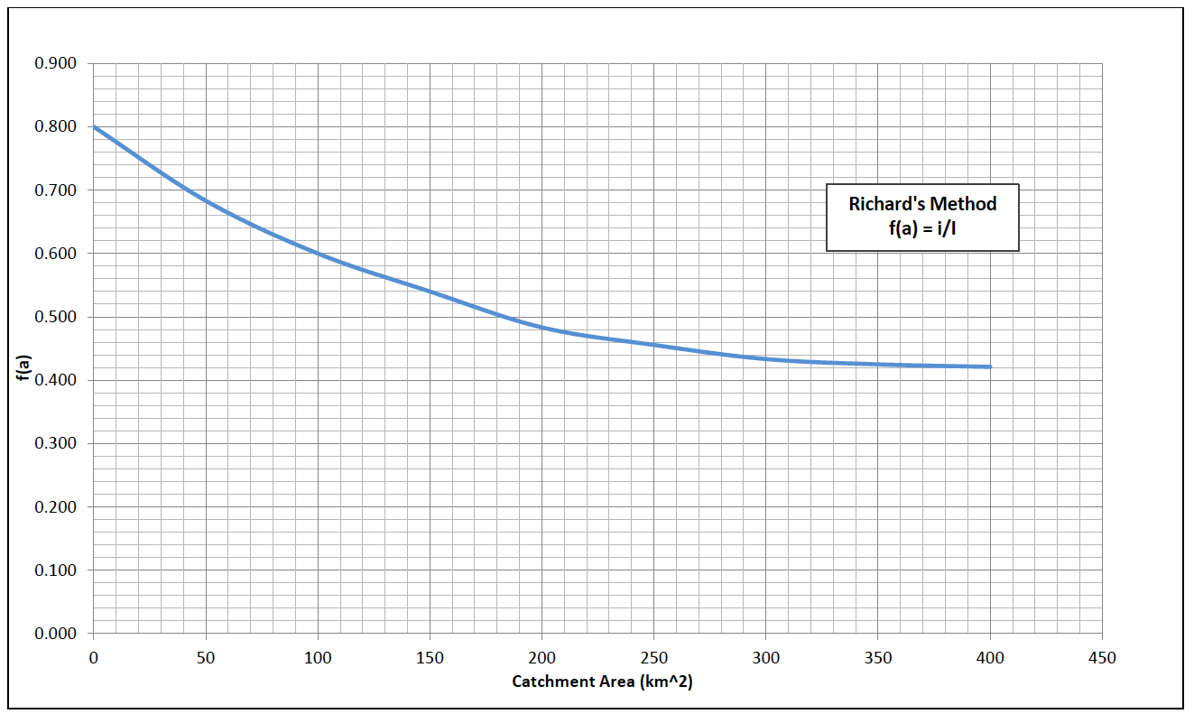
Figure 8-6: Rainfall Intensity Factor, Richard's Method
Equation 8-4: i = $I_{max}$ . f(a)
Where:
i = average rainfall intensity [mm/hr] over the catchment
$I_{max}$ = maximum rainfall intensity = $\frac{R}{TC+1}$ [mm/hr]
f(a) = ratio of the average rainfall intensity (i) to the maximum rainfall intensity ($I_{max}$) over the catchment area, obtained from Figure 8-6.
Finally the rational formula is used to calculate the expected maximum flow as shown in Equation 8-5.
Equation 8-5: $Q_p = \frac{K_r . i . a}{3.6} $
Where:
$Q_p$ = peak flood flow [$m^3$/s] with return period equal to that of the selected storm and
i = average rainfall intensity [mm/hr] over the catchment
a = the area of the catchment [$km^2$].
8.10.3 TRRL and East African Flood Prediction Method
The TRRL and East African Flood Prediction Model as described in the TRRL Laboratory Report No. $623^4$. It can be used for catchments where Richards Method is not considered appropriate.
8.10.4 SCS Method
The US Soil Conservation Service (SCS) Rainfall/Runoff Model was developed in the USA and is widely used globally. The model uses rainfall data, catchment and soil conditions to estimate discharge.
The SCS Model assumes that there are two stages in modelling the response to rainfall:
- Initial retention of rainfall.
- Infiltration and runoff.
During Stage 1, there is no runoff. Once the “Initial Retention” storage is filled, Stage 2 commences. Both stages are functions of land use, soil infiltration capacity, depression storage, and antecedent soil moisture.
Initial Retention
The Initial Retention is computed by Equation 8-6 and Equation 8-7
Equation 8-6: $I_a$ = 0.2S
Equation 8-7: S = 254($\frac{100}{CN}$ - 1)
Where:
$I_a$ = Initial Retention [mm]
S = Potential Maximum Retention [mm] calculated using Equation 8-7
CN = Runoff Curve Number as established from Table 8-9.CN values are published for various land cover conditions, various antecedent soil conditions and for various hydrologic soil groups.
Soil Group Classification
SCS developed a soil classification system that consists of four soil groups whose soil characteristics are provided in Table 8-8.
Table 8-8: SCS Method Hydrologic Soil Groups
Hydrologic Soil Group Drainage characteristics Group A Deep sand, deep loess, aggregated silts Group B Shallow loess, sandy loam Group C Clay loams, shallow sandy loam, soils low in organic content, and soils usually high in clay Group D Soils that swell significantly when wet, heavy plastic clays, and certain saline soils (Source: McCuen, US SCS)
Curve Numbers for Different Cover Complexes and Hydrological Soil Groups
Table 8-9 provides curve numbers (for AMC II conditions) for different cover conditions and soil groups.
Table 8-9: Runoff Curve Number (CN) for AMC IIHydrologic Soil Group Land use Detail A B C D Cultivated land Without conservation treatment 72 81 88 91 Cultivated land With conservation treatment 62 71 78 81 Pasture or rangeland Poor condition 68 79 86 89 Pasture or rangeland Good condition 39 61 74 80 Meadow Good condition 30 58 71 78 Wood or forest land Thin stand, poor cover, no mulch 45 66 77 83 Wood or forest land Good cover 25 55 70 77 Open spaces, lawns, parks Good condition : grass cover >75% of areas 39 61 74 80 Open spaces, lawns, parks Fair condition : grass cover 50 - 75% of areas 49 69 79 84 Commercial and business areas ≈ 85% impervious 89 92 94 95 Industrial areas ≈ 72% impervious 81 88 91 93 Roads Paved 98 98 98 98 Roads Gravel 76 85 89 91 Roads Dirt 72 82 87 89 Fallow Bare soil 77 86 91 94 Fallow Crop residue 76 85 90 93 Fallow Good 74 83 88 90 Row crops Poor 72 81 88 91 Row crops Good 67 78 85 89 Woods - Bush Poor 57 73 82 86 Woods – Bush Fair 43 65 76 82 Woods – Bush Good 32 58 72 79 (Source: McCuen, US SCS)
In catchments with different cover conditions, it is possible to develop a Curve Number (CN) representative of the catchment based on an area weighted method in which the curve numbers for different parts of the catchment are established and the respective area determined.
Antecedent Soil Moisture Condition
The antecedent moisture factor has a significant effect on runoff and SCS developed three antecedent soil moisture conditions, as shown in Table 8-10. AMC II is typically applied.
Table 8-10: Antecedent Moisture Condition
Antecedent Moisture Condition (AMC) Soil Condition AMC I Driest soil conditions (i.e. wilting point) AMC II Average conditions AMC III Wettest soil conditions (i.e. > field capacity) Curve Number Estimation
Typical runoff curve numbers are tabulated in Table 8-8 for AMC II (average conditions). These can be adjusted according to the moisture conditions (Haith 1985). AMC III conditions would apply for periods of high rainfall or for flood analysis where the five day antecedent precipitation would be expected to exceed 53mm. AMC I would be applicable for dry conditions where five day antecedent precipitation is less than 35 mm.
Equation 8-8:
CN(III) = $\frac{CN(II)}{(0.4036 + 0.0059CN(II))}$
Equation 8-9:
CN(I) = $\frac{CN(II)}{(02.334 - 0.01334CN(II))}$
Where:
CN(I) = curve number under AMC(I) conditions
CN(II) = curve number under AMC(II) conditions
CN(III) = curve number under AMC(III) conditionsDischarge Estimation
The runoff is computed by Equation 8-10:
Equation 8-10:
Q = $\frac{(P-0.2S)^2}{(P+0.8S)} \times A \times 10^6$
Where:
Q = discharge [mm]
P = Storm catchment averaged rainfall [mm]
S = Potential Maximum Retention [mm] calculated using Equation 8-7
A = Catchment area [$Km^2$]
8.10.5 Flood Frequency Analysis Based on Discharge Data
Whenever possible, the determination of the expected peak flows should be based on actual and accurate stream flow data. When such data are available, a flood frequency analysis based on the annual maximum discharge series should be can be undertaken. Care should be taken to use the hydrological year (October – September), not the calendar year (January – December) to establish the annual maximum series. An open source statistical software (e.g. Easyfit) can be used to fit different probability distributions to the annual maxima data series. Care should be taken to select probability distributions appropriate for discharge analysis e.g.
- Gumbel – EV Type ;
- Frechet - EV Type II;
- Weibul - EV Type III;
- Log-Pearson Type III;
- Log Normal Distribution;
- Wakeby Distribution.
8.11 Probable Maximum Flood (PMF)
The analysis of probable maximum flood is not essential for small dams considered in this manual. However in the event that the small dam poses a significant risk to downstream populations, the PMF analysis may be required to provide additional information for the spillway design.
The estimation of the probably maximum flood requires an estimate of the probable maximum precipitation based on the annual maximum rainfall series. The Hershfield Formula5 (Equation 8-11) can be used to calculate the PMP or values can be obtained from the isohyetal map of PMP in the NWMP (1992).
Equation 8-11:
PMP = P + K.Sp
Where:
PMP = Probable Maximum Precipitation
P = Mean of Maximum Annual Precipitation
Sp = Standard Deviation
K = Number of Standard Deviations that must be added to the mean to obtain PMP
K is obtained from Figure 8-7
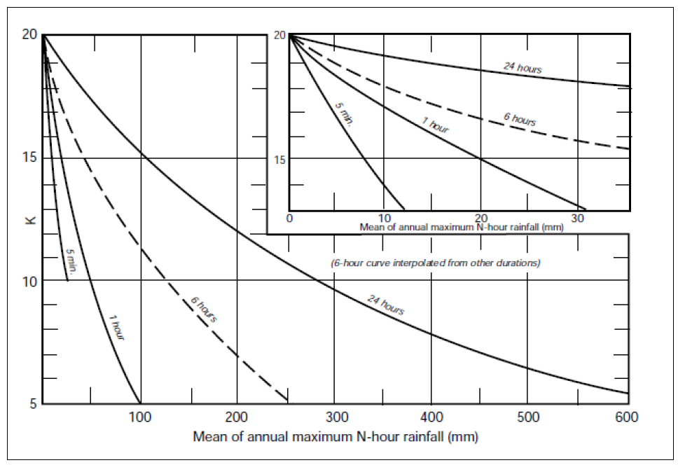
Figure 8-7: K as a Function of Rainfall Duration and Mean of Annual Maximum Series
The National Water Master Plan (MWI 1992) presents a relationship between PMF, PMP and Catchment Area.
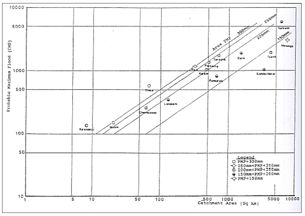
Figure 8-8: Relationship between PMF, PMP, and Catchment Area
8.12 Determining Storage Requirements
The total storage required is the summation of the active and dead storage requirements.
In general the active storage should be sufficient to meet the demand (with an acceptable level of reliability) and losses for the duration of the dry season until there is inflow in the rainy season to refill the storage.
In the semi-arid and arid areas, it cannot be ruled out that one of the two usual rainy seasons does not yield sufficient runoff to replenish the reservoir storage, and that consequently long periods will have to be catered for.
However, for most rivers in the rural areas, no stream flow data might be available and an educated guess towards the length of the dry period will have to be made. Table 8-11 presents estimates of the length of the dry season for different rainfall regimes from MWI (2005). Interviews with local residents will also provide good information regarding the length of the dry period.
Table 8-11: Estimated Length of Dry Period
| Mean Annual Rainfall (mm) | Length of Dry Period (month) |
|---|---|
| 1200-1000 | 5 |
| 1000-800 | 7 |
| 800-400 | 9 |
| <400 | 11 |
In case no precipitation data from rainfall stations in the considered catchment area is available, comparison should be made with other similar catchments.
In the case of reservoirs for which the principal purpose is to provide water for nomadic populations and their livestock, it is not always desirable to create reservoirs where water is available on a year round basis. This might provoke a considerable concentration of people and livestock in the concerned area, in turn generating problems such as overgrazing and ecological degradation of the catchment area. The notion of “storage reliability" as outlined above is therefore not applicable in these cases and the storage structure should be designed to provide water for only part of the dry season.
8.12.1 Dry Season Storage
In such cases the graphical method outlined below can still be useful to evaluate the following:
- Length of the dry period for which a given level of supply can be maintained;
- Which level of supply can be maintained during a given dry period;
- Assessing the relative importance of the evaporation losses compared to the water consumption.
The simplified graphical method for determining reservoir storage capacity is illustrated in Figure 8-9.
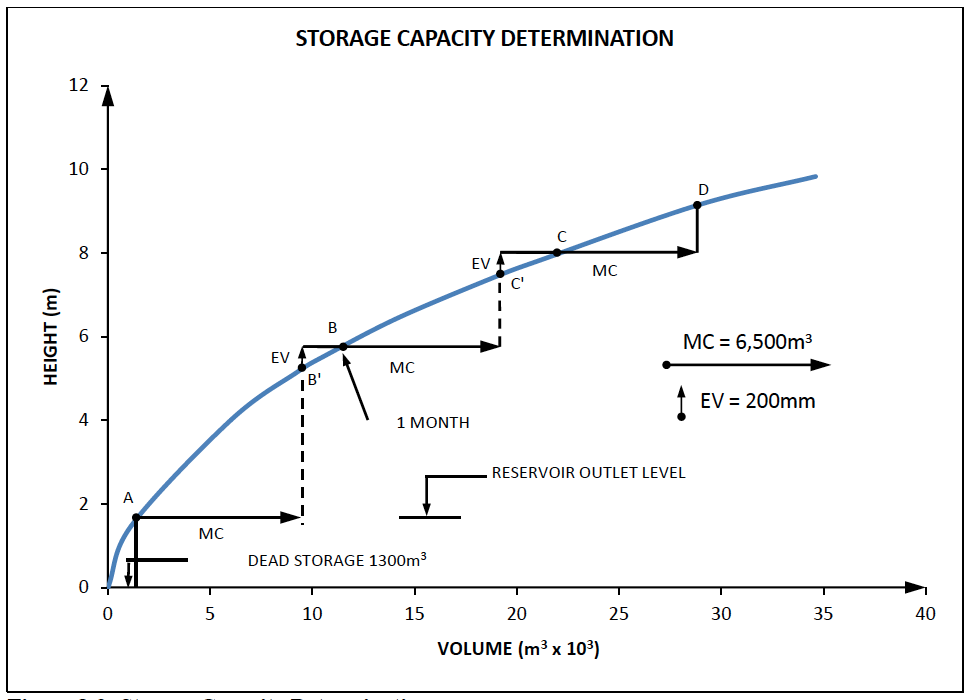 Figure 8-9: Storage Capacity Determination
The following input parameters are required:
- A Height / Storage Capacity Curve of the reservoir;
- Monthly water demand or anticipated monthly water consumption (MC);
- The volume taken up by the "Dead Storage" in the reservoir. This is equivalent to the volume of water stored below the level of the lowest draw-off, and is usually very small for the type of dams and draw-off-systems considered;
- Monthly flow (if any) in the river during the concerned dry period;
- Monthly evaporation (EV) losses. Averages based on annual figures obtained from NWMP 1992 can be used as a general guideline;
- The quantity of sediment expected to be retained by the reservoir during its design life period (See Section 8.13).
The graphical method proceeds as follows: (See Figure 8-9)
- The level (or alternatively the storage volume) corresponding with the dead storage is set out from point O on the Height/Storage Capacity curve (Point A).
- From point A, the monthly water consumption (MC) - where applicable reduced by the monthly inflow in the reservoir - is set out horizontally, and transported back to the curve (point B'). From point B', the monthly evaporation (EV) is set out vertically and transported back to the curve (Point B). Point B indicates the storage requirements for one month or for the last month of the dry period, excluding provisions for sediment storage.
- From point B, the above procedure is repeated, until eventually the storage required to cater for the whole length of the dry period is established.
Since evaporation losses are expressed in millimetres of height, the volume of water lost through evaporation is directly related to the surface of the reservoir. The outlined method determines the evaporation losses at the beginning of each month, and therefore slightly over-estimates the losses. However, this compensates for a number of other minor water losses (infiltration, seepage etc.) which are not taken into account. It must be clear that from the point of view of evaporation losses, for a given storage capacity, deep reservoirs are preferable to shallow ones.
In addition to the storage requirements obtained as outlined above, it is common practice to provide some additional reservoir capacity to cater for sediment storage.
8.12.2 Mass Diagram Analysis
A quick check should be made to ensure that the sum of the average annual water demand (including evaporation and seepage losses) in cubic metres per day is less than the mean annual flow [$m^3$/day] as it is not possible to extract more water from the catchment than the estimated inflow.
The Rippl Curve (Loucks et al, 1981) provides a graphical method to establish the required storage based on average monthly values for demand, evaporation and seepage losses. The analysis is more easily done using the mean monthly inflows. The procedure is as follows:
- Plot the cumulative mean monthly inflow volume for 24 months by repeating the 12 month average monthly inflow sequence;
- Draw a straight line tangential to the cumulative inflow curve. This line should have a gradient equal to the combined average monthly evaporation, seepage and demand ($m^3$/month);
- Establish the maximum difference between the cumulative mean inflow line and the cumulative demand line. This difference represents the active storage required in cubic metres.
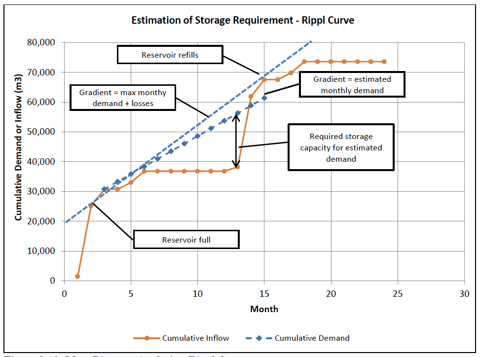
Figure 8-10: Mass Diagram Analysis - Rippl Curve
The method provides a quick way to ascertain the scale of storage that is required. The shortcoming with the Rippl curve methodology as presented above is that it uses mean monthly flow values and a uniform demand value.
If monthly demand values vary, then a modification is to plot the cumulative difference between monthly inflow and the combined monthly release (demand, evaporation and seepage).
8.12.3 Sequent Peak Analysis
The Sequential Peak Method (Loucks 1981) provides an alternative graphical method to establish the required storage. A quick check should be made to ensure that the sum of the average annual water demand (including evaporation and seepage losses) in cubic metres per day is less than the mean annual flow [$m^3$/day] as it is not possible to extract more water from the catchment than the estimated inflow.
Sections 8.8 and 3.3 provide the methodologies for estimating the inflow to the storage structure and the demand and losses (evaporation and seepage) respectively.
The analysis is more easily done using the mean monthly demand and flow values. A data set should be established for a 24 month period by repeating the sequence of mean monthly values. This takes care of the case where the critical sequence occurs across the end of the first 12 month period.
This method tracks the positive values of the storage required in any given time period which is the sum of the storage required at the end of the previous time period plus the demand (and losses) minus the inflow. This can be represented mathematically as shown in Equation 8-12.
Equation 8-12:
$\mathbf{K_t = Max[(D_t + E_t + S_t - Q_t + K_{t-1}), 0]}$
Where:
$K_t$ = storage required at the end of time period t [$m^3$]. $K_0$ is equal to zero
$D_t$ = Demand in period t (inclusive of environmental release) [$m^3$]
$E_t$ = Evaporation losses in period t [$m^3$]. Note that this equals zero for a covered tank
$S_t$ = Seepage losses in period t [$m^3$]. Equals zero for a covered tank and lined pan
$Q_t$ = Inflow in period t [$m^3$].
The storage volume required ($K_{max}$) is the maximum value of $K_t$ across the period of analysis.
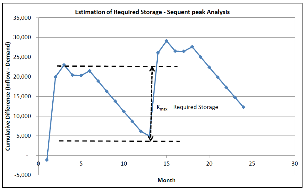
Figure 8-11: Example of Sequent Peak Method
Some consideration needs to be given to the values for evaporation losses ($E_t$) and seepage losses ($S_t$) in each time period because the value is actually dependent on the water depth in each given time period. Section 3.3.10 and 3.3.11 provide a method for estimating a maximum value for these parameters which can be used across all the time periods.
8.12.4 Reservoir Simulation
Computer simulation models, based on a daily or monthly time step, can be used to simulate the inflow, spills, demands and losses of a reservoir based on a simple water balance approach. A computer simulation model provides a useful tool to analyse the required storage, yield reliability and release rules. Various open source reservoir simulation models are available including HEC-ResSim.
The basic water balance equation for reservoir simulation as a daily time-step is shown in Equation 8-13.
Equation 8-13:
$\mathbf{ S_{t+1} = S_t + P_t + I_t - E_t - Seep_t - R_t - Spill_t}$
Where:
$S_t$ = Storage on day t [$m^3$]. This is established from the HVA curve for the given depth on day t
$P_t$ = Precipitation on reservoir area on day t [$m^3$]. The area on day t is a function of the depth on day t which is determined from the HVA curve.
$I_t$ = Inflow into reservoir on day t [$m^3$].
$E_t$ = Evaporation from reservoir surface area on day t [$m^3$]. The area on day t is a function of the depth on day t which is detemined from the HVA curve.
$Seep_t$ = Seepage from reservoir on day t [$m^3$].
$R_t$ = release from reservoir on day t [$m^3$]. This may include releases to meet environment flow requirements and to meet water demand.
$Spill_t$ = Spillway overflow on day t [$m^3$]. This is a function of the water depth above spillway crest and the hydraulic properties of the spillway control and channel.
It should be noted that the water balance equation can be modified appropriately for use with a monthly time-step.
A simulation model provides an easy tool for scenario analysis which may include:
- Establishing the expected length of the filling period;
- Reservoir performance in exceptionally dry or wet periods;
- Reservoir performance under different release rules;
The reservoir performance can be assessed against different indicators for different objectives which may include:
- Drawdown;
- Reliability of meeting specified releases;
- Spillway flows.
Use of a reservoir simulation model requires some consideration of the initial conditions. If the analyst aims to analyse the normal operating conditions of the reservoir, then it is advisable to start the simulation with the reservoir storage level at a level appropriate to the starting time period. For example, if the simulation starts at the end of the rainy season, then the storage level could reasonably be expected to be at the spillway level.
8.13 Sedimentation
Every river and water course carries some suspended sediment and moves larger solids along the stream bed as bed load. When sediment-laden water reaches a reservoir, the larger suspended particles and most of the bed load are deposited as a delta at the head of the reservoir (See Figure 8-12). Smaller particles remain in suspension longer and are eventually deposited farther down the reservoir or may even pass the dam with water discharged through the spillway.
The design of a reservoir should consider the need for and arrangements for sediment scour works. The first step is to estimate the extent of sediment inflow into the reservoir and the impact that may have on the functionality of the reservoir. If the sediment inflow is high, then a mechanism to remove the sediment, including the option of sediment scour works, can be considered. It should be noted that removal of sediment by means of a scour pipe is not straightforward because the heavy sediments lie at the head of the reservoir and sediments consolidate over time.
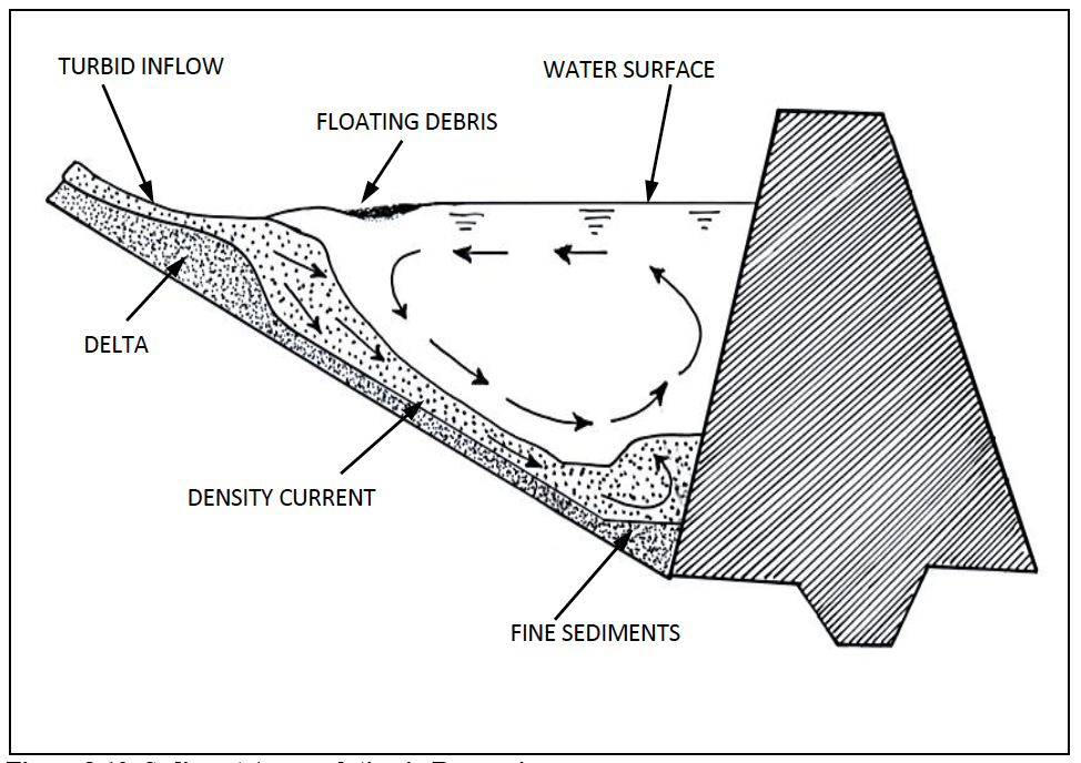
Figure 8-12: Sediment Accumulation in Reservoirs
The quantity of sediment transported in a river depends on many factors that include the rate of erosion within the catchment area, sediment deposition within the catchment, and flow conditions in the water course. The rate of erosion of a particular catchment may vary from flood to flood, with variations in rainfall intensity, soil condition, and vegetal development.
Especially in the arid and semi-arid areas sedimentation is generally of considerable significance in the design, construction and rehabilitation of small dams and pans in Kenya.
Some representative figures for the sediment yield of catchments in Kenya are given in Table 8-12. These figures can be considered as conservative values of sediment yield.
Table 8-12: Indicative Sediment Yields
| Erosion Rate | Sediment Yield ($m^3$/$km^2$/year) |
|---|---|
| Low | 500 |
| Moderate | 1000 |
| Heavy | 1500 |
source: MWI 2005
The trap efficiency of a reservoir is defined as the percentage of in flowing sediment which is retained in a reservoir. The trap efficiency is a function of the ratio of reservoir capacity to total inflow. Hence, the trap efficiency of a reservoir decreases with age as the reservoir capacity is reduced by sediment accumulation. Figure 8-13 may be used to estimate the percentage of the annual sediment load which a reservoir will trap.
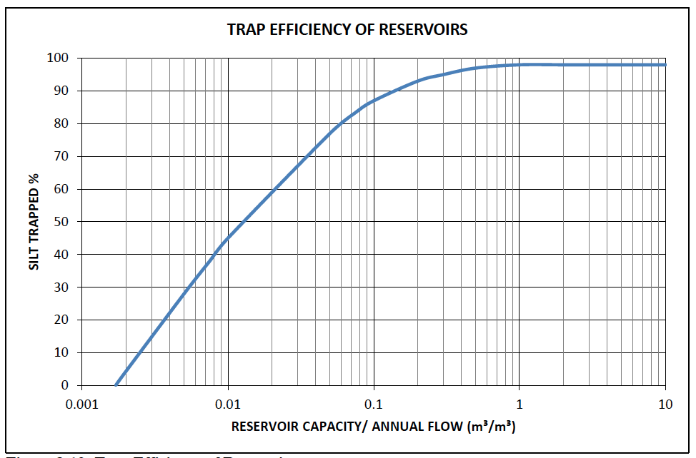
Figure 8-13: Trap Efficiency of Reservoirs
Sediment inflow to a reservoir may be reduced to a certain extent by the use of soil conservation methods within the catchment area as outlined in Chapter 7 (Erosion Control and Catchment Conservation).
In cases were heavy sedimentation is expected, and where no alternative dam location can be found, the possibilities of constructing an upstream silt trap should be examined. However, in order to fulfil their function properly silt traps require regular maintenance (emptying).
8.13.1 Dead Storage
The dead storage requirement is a function of the expected volume of sediments and the need for permanent water within the reservoir, for fish keeping or other ecological factors.
A reasonable estimate of the sediment volume that would accrue in the reservoir across the life span of the structure can be made using the details described above. This value should provide a guide to the extent of dead storage required. The dead storage level can be determined from the height-volume-area (HVA) curve for the dam site. This level will define the level of any offtake works.
8.14 Environmental Flows
The Reserve is defined by the Water Act 2002 as the quantity and quality of water required:
- to satisfy basic human needs for all people who are or may be supplied from the water resource; and
- to protect aquatic ecosystems in order to secure ecologically sustainable development and use of the water resource.
The design of a dam or reservoir located on a water course will need to comply with the requirements of the Reserve as specified in the WRM Rules (2007). The Rules state that the flow shall exceed the $Q_{95}$ or the flow that is exceeded 95% of the time, as defined by a naturalised flow duration curve. This value can be extracted from the FDC (See Section 8.9).
The environmental releases should be sufficient to meet human and ecological demands downstream. These may require a critical analysis of the release requirements with respect to water quality (physical, chemical and biological characteristics), and the quantity, pattern, timing, and reliability of in-stream flow downstream of the reservoir.
The water quality of reservoir releases, drawing water from the lower fraction of the reservoir, typically has low dissolved oxygen levels. Turbulence in the flow downstream of the reservoir will return the DO level to steady state conditions. This process can be assisted with structural features, such as energy dissipaters, to increase the turbulence and aeration of the releases.
The quantity, timing, and reliability of the releases can be addressed by establishing a schedule of release that reflects the natural pattern of flow. This can be partially achieved by establishing the $Q_{95}$ for each month. This would provide a specific release for each month that reflects the natural pattern. Consequently the design of the scour pipe should be sufficient to release the maximum monthly $Q_{95}$.
Consideration should be given on how to ensure minimum downstream floods as this is part of the natural hydrological pattern. If the ratio of reservoir volume to mean annual flood volume is less than 0.5, then it can be expected that natural flood events will occur. For values greater than 0.5, the reservoir may eliminate or drastically reduce downstream floods which could affect recharge of river banks and flood plains, and sediment transport along the water course. It may therefore be necessary to periodically provide a high volume short duration release. The requirements for this type of release should be determined on a case by case basis in consultation with WRMA.
In the case of online reservoirs on an ephemeral water course, the timing and quantity of environmental releases requires some consideration. In order to be compliant with the WRM Rules (2007), there should be a release whenever there is inflow into the reservoir. The quantity of the release will depend on the water level in the reservoir. This schedule of release should be established in consultation with WRMA and the local WRUA.
A sample reservoir release rule is presented in Table 8-13 in which the maximum environmental release ($QE_{max}$) may be determined as the $Q_{95}$ if discharge records exist, or flow sufficient to result in open water for at least 5 km downstream or such other distance as agreed by WRMA.
Table 8-13: Sample Reservoir Release Rule for Online Reservoir on Ephemeral Water Course
| Status of Inflow to Reservoir | Status of Water Level in Reservoir | Environmental Release | Comment |
|---|---|---|---|
| Flow | < 50% | Equal to the inflow up to a maximum of 25% of $QE_{max}$ | Scour pipe is set to release 25% of $QE_{max}$. |
| Flow | > 50% | $QE_{max}$ | Scour pipe is set to release 100% of $QE_{max}$. |
| No Flow | < 50% | 0 | |
| No Flow | > 50% | 25% of $QE_{max}$ | Implies reservoir is increasing reliability of downstream flows |
The analysis of the Reserve for an offline storage structure will focus on the design of the river intake works to ensure that this meets the Reserve flow requirements and compliance with the WRM Rules (2007) with respect to the quantity and timing of authorised abstractions.
It should be noted that the actual releases from a reservoir in any given month may be a function of two components:
- Environmental flow requirements as determined from the discussion above;
- Releases to meet authorised downstream abstractions.
9 Site Surveys And Investigations
Site survey work for small scale storage encompasses much more than just topographical survey work. It involves testing and sampling soils and available materials as well as undertaking preliminary subsurface investigations.
Other less technical site survey work can be carried out and is dealt with in other chapters. See Chapter 10 for Reconnaissance Survey Details and Chapter 6 for Resettlement Concerns.
There may be long periods between the initial survey work and the decision to proceed with a project. Different teams of people may be involved with the survey, the design and then the supervision of the project, so all survey work must be accurately recorded with sufficient details to allow anyone to make use of it at any stage in the project.
Depending on the size of the proposed reservoir, the initial survey team may consist of a design engineer, a surveyor, a hydrologist and a geotechnical engineer. Survey work may be carried out in stages with a preliminary survey to establish initial site conditions and a final survey to provide detailed information.
Additional information on site surveys and investigations can be found in Small Dams and Weirs in Earth and Gabion Materials, (Charman J. et al., 2001), Design and Construction of Small Earth Dams, (Nelson K. D., 1985) or Water from Ponds, Pans and Dams, (Lindqvist A.K, 2005)
9.1 Topographical Survey of Storage Site
The topographical survey work output should be a set of drawings that provides all topographical information and details required to carry out the design of the dam, pan or water conservation structure. Historically grid based survey techniques were used. While still very effective, especially in areas with dense bush or tree cover, they are not entirely necessary with modern survey equipment.
The most important point is to make sure that any site survey has sufficient survey data to provide confidence in the contour maps produced.
A survey must extend a considerable distance above the expected crest level to allow for looking at overtopping scenarios and to allow for spillway planning and positioning decisions. In general, a survey that extends 5m in elevation above the proposed embankment crest level is desirable.
Surveys must extend a considerable distance downstream of the planned embankment to allow for the spillway return channel to be positioned correctly. In general, a minimum of 50m downstream of the proposed embankment alignment is permissible and at least 150m is desirable.
Surveys should also cover all expected borrow areas in sufficient details to allow for accurate borrow material calculations.
In the case of pan and lagoon surveys, it is often necessary to survey a considerable distance upstream (or uphill) from the proposed structure to ensure that an inflow channel that captures runoff can be constructed.
In the case of sand and sub-surface dam site surveys, survey data should not only include topographical information but should estimate subsurface conditions collected through the use of steel probes.
It is the responsibility of the design engineer to specify the limits of the survey work to be carried out.
9.1.1 Pre-Survey for Site Selection Purposes
In cases where a pre-survey has to be organised in order to select the most economical location of the dam from the topographical point of view, the following information should be obtained for each prospective dam site:
- One cross-section of the valley at the location of the prospective dam axis. It is recommended that for this cross-section measurements be taken at intervals not exceeding five (5) metres.
- A longitudinal profile of the river, with three (3) to five (5) additional cross-sections taken along the longitudinal profile. The number of cross-sections should be decided as a function of the length of the reservoir. The longitudinal profile must extend up to the expected water level and if possible should extend approximately 5m (vertical distance) above the expected water level.
During initial site visits, the GPS coordinates for the site should be recorded. The map datum used in the GPS should also be recorded. With this information, the site can be located on existing maps and within Google Earth.
If a detailed pre-survey is not possible, either a tape measure or an Abbney level and hand held EDM (preferably with an inclinometer) can be used to determine estimated embankment lengths and heights as well as longitudinal slopes along the valley.
The pre-topographical survey visit should also collect information relevant to an environmental scoping study (See Chapter 6 and Chapter 10 for more information). This can include information on stakeholders in the area, landowners likely to be affected by the project, assets within the project area, downstream infrastructure etc.
9.1.2 Final Survey of the Storage Site
The final survey of the storage site should allow the elaboration of contour maps as specified in Table 9-1.
Table 9-1: Specification for Topographical Maps
| RESERVOIR AREA | DAM & SPILLWAY AREA | |
|---|---|---|
| SCALES | 1/500 to 1/1000 | 1/250 |
| CONTOUR INTERVALS | 1.0m to 2.0m | 0.5m to 1.0m |
For the final survey, it is recommended that the following guidelines be adhered to in order to obtain all required information for the design of the dam:
- The dam axis and the dam crest level shall be indicated by the designer. The highest (upper) contour line to be surveyed should be taken as 5m above the crest level of the embankment. The upper contour line for the site must close in the final survey drawings.
- The survey of the dam and spillway area shall cover an area of 200 metres upstream and downstream of the dam axis, and should be extended for a distance of 15 metres from the upper contour. For this area a topographical map of 1/250 scale should be prepared with contour intervals not exceeding one metre. For the rest of the reservoir area, the scale of topographical maps can be 1/500 or 1/1000, while contour intervals should not exceed one (1) metre.
- Four (or more) solid concrete bench marks shall be established by the survey team. Figure 9-1 shows details of a possible type of bench mark. Two of these bench marks will indicate the dam axis alignment. They should be located at a horizontal distance of at least 10 (ten) metres from the upper contour level.
-
If surveying using a grid system, an indication towards the grid (or cross-section) distances to be used for the final survey is given in Table 9-2. If surveying without establishing a grid, a higher point density should be established within the proposed embankment footprint and within the proposed spillway location. The density of points should be sufficient for an accurate contour map to be produced.
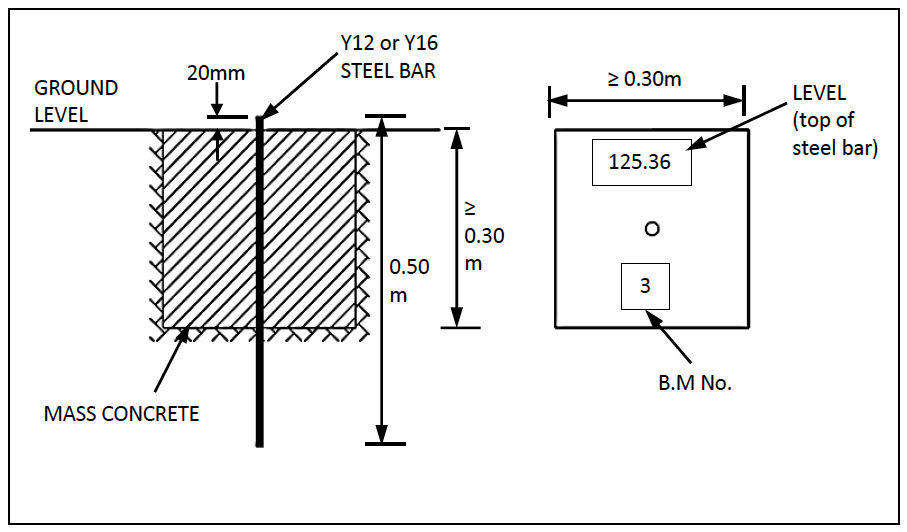
Figure 9-1: Survey Benchmark
Table 9-2: Suggested Grid Spacing for Survey Work
DISTANCE FROM DAM AXIS GRID DISTANCE <50m (up & downstream) 5m to 10m 50m to 150m (up & downstream) 25m 150m to 500m (upstream only) 50m >500m (upstream only) 100m - Within the survey area covered, all man-made structures and cultivations should be indicated with their ownership. River crossings (bridges, pipelines, etc.) within 300 metres downstream of the dam axis or situated lower than 2 metres above the upper contour line on the upstream side of the reservoir, should also be indicated.
- All surveys should be “closed out” to confirm the level of accuracy of the survey measurements. When this is not done, it should be noted and the reasons for not doing it should be clearly presented.
- All contours below the high flood level must be closed contours (there must not be areas that will be flooded that have not been surveyed. It is often difficult to close high flood contours as it may require surveying up the watercourse a considerable distance past the normal water level.
Figure 9-2 shows a summary of the final survey guidelines for prospective dam sites for small earth dams.
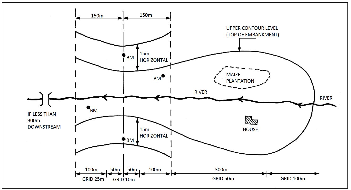
Figure 9-2: Summary of Final Survey Guidelines for a Dam Site
For pans and lagoons a 10m grid should be used in the areas where embankments will be placed. A 25 to 50 meter grid can be used in all other areas. The survey area must extend at least 25 meters horizontally beyond the final extent of any expected earthworks. The survey should extend far enough upstream to ensure that an inlet channel can be constructed and to provide information relevant to silt trap construction.
For sand dams and subsurface dams, the survey should be most dense (10m grid or finer) in the area where the wall will be constructed. It can be less dense in the upstream areas. It should capture the positions and relative heights of river banks (i.e. height above the stream bed) as this information is needed during the design process.
For rock catchments, the survey should cover the entire rock face with dense grids in any localized depressions. Rock catchment construction can often extend catchments through the use of training walls to direct water flow. It is important that the survey covers areas outside of the natural catchment area if training walls are to be used. When in doubt as to the required extents of the survey capture as much information as possible on the entire rock face, even if it means only a sparse (50 to 100m) grid can be used.
9.2 Survey Equipment and Software
A variety of modern survey equipment is available and, with careful choosing, can greatly simplify the survey tasks associated with small earth dam design and construction.
Table 9-3 gives a brief summary of types of survey equipment and their main uses. It is not an exhaustive list and other equipment may be used as determined by the surveyor and/or design engineer.
Table 9-3: Survey equipment and suggested Uses
| Equipment | Main Uses | Notes |
|---|---|---|
| Abney Level | Initial site selection | Hand held, gives initial estimates for levels and slopes |
| Barometric Altimeter | Initial site selection | Can be accurate for relative changes in elevation and for checking handheld GPS elevations. |
| Handheld EDM (electronic distance measure) | Initial site selection and volume estimation | Available with slope readouts. Distance measure between 100m and 500m. |
| Handheld GPS | Initial site selection, locate site on contour map or in Google Earth. Can measure areas. | NOT SUITABLE FOR ACCURATE ELEVATION MEASUREMENT. |
| Dumpy levels | Mostly suitable for site layouts and construction supervision. | Can be used for site surveys on small (less than 100m x 100m sites) |
| Theodolites | Suitable for survey work for most sites | Requires lots of mathematical calculations |
| Total Stations | Suitable for survey work for all sites | Requires at least two benchmarks to ensure all measurements use same coordinate system. |
| Survey quality GPS | Suitable for survey work of sites. Not suitable for layout work | Requires only one benchmark. Not suitable for sites with dense tree cover. |
| Real Time Survey Quality GPS | Suitable for survey work of sites. Suitable for layout work | Requires only one benchmark. Can be used in sites with some tree cover. |
Along with modern survey equipment, there is a variety of modern computer software to assist in survey tasks associated with the design and construction of dams, pans and other small water conservation structures.
Table 9-4 lists common software and suggested uses. Again, this is not an exhaustive list and additional software may be required for specific design work.
Table 9-4: Typical Software Used in Survey and Design of Small Dams
| Software | Main Uses | Notes |
|---|---|---|
| AutoCAD Civil 3D | Survey data manipulation, contour generation, calculation of volumes (earth and storage) | Can be expensive, other similar software is available. Can be difficult to learn (PROGECAD….) |
| Microsoft EXCEL | Survey data manipulation. Repetitive calculation | Any spreadsheet software will work. |
| SURFER | Digital terrain modelling. Works well with excel based data sets and allows contour generation, volume calculations etc. | Fairly inexpensive and very easy to learn |
| ARC GIS | Larger scale mapping, catchment examinations | Can be expensive and difficult to learn. |
| Google Earth | Initial site examinations, catchment characteristics, relevant infrastructure | Requires accurate positioning data (from hand held GPS is more than sufficient) |
| HECRAS | Used for flood estimation and routing | Requires detailed survey data for river channels. |
9.3 Height-Volume-Area Relationship Curve
The height-volume-area relationship (“HVA curve”) or storage-area curve is developed from the survey data. The HVA curve provides an important site specific information on the relationship between height (or water depth), volume, and area. In addition to the layout map, the HVA curve is perhaps the most important output from the site survey work as the data it presents is used to evaluate different inflow, outflow and storage scenarios during the design work.
Convention dictates that the water depths or embankment heights are plotted on the vertical axis and the corresponding areas and volumes are plotted on the horizontal axis. This can be achieved by plotting the volumes on the primary horizontal axis (at the bottom of the graph) and the areas on the secondary horizontal axis (at the top of the graph) which is reversed as shown in Figure 9-3.
9.3.1 Developing the HVA Curve
Developing the HVA curve requires a site contour map drawn to scale. The contour map is the primary output from the site survey work and provides all required information for developing the HVA curve.
If the contour map is only available in a paper copy, the following procedure should be followed:
- Make a copy of the map.
- Lay out the centreline of the proposed embankment on the map.
- Lay out an appropriately scaled grid on the map. The grid can be aligned with a compass bearing or with the proposed centreline or with any other relevant feature on the map. It is best to use a uniform grid spacing (10m x 10m or 20m x 20m….). The actual grid size is determined by the size of the proposed storage (for a large project, a 50m x 50m grid may be reasonable, for a small project, a 5m x 5m grid may be sufficient). Once a grid is laid out, make several additional copies of the map. In general, for a 5m deep storage structure make 5 copies, for a 10 meter deep structure make 10 copies.
- Starting with the lowest contour upstream of the proposed centre line, determine the “flooded” area between the contour and the centre line. This figure is the area that would be flooded if water filled the valley up to that specific contour level.
- Continue working up one contour at a time, determining the flooded area for each contour. It is usually easiest to do this on a clean map copy and to determine areas by counting grid squares and then multiplying by the area of a single grid square. For example, with a 10m x 10m grid, if the flooded area took up 25.6 grid squares, the final flooded area would be 25.6 grid squares x 100m2/grid square which is 2,560 square meters.
- Establish a table as shown below. In this table, the contour at 2,134 was not closed and it was not possible to get a flooded area figure from the contour map.
Table 9-5: Typical Elevation and Area Table
| Elevation (m) | Water Depth (m) | Flooded Area ($m^2$) |
|---|---|---|
| 2,127.50 | 0 | 0 |
| 2,128.00 | 0.50 | 1,500 |
| 2,128.50 | 1.00 | 5,241 |
| 2,129.00 | 1.50 | 8,614 |
| 2,129.50 | 2.00 | 12,691 |
| 2,130.00 | 2.50 | 17,703 |
| 2,130.50 | 3.00 | 25,181 |
| 2,131.00 | 3.50 | 31,983 |
| 2,131.50 | 4.00 | 38,883 |
| 2,132.00 | 4.50 | 48,916 |
| 2,132.50 | 5.00 | 57,545 |
| 2,133.00 | 5.50 | 68,442 |
| 2,133.50 | 6.00 | 81,579 |
| 2,134.00 | 6.50 |
If the contour map is available in a soft/CAD copy, then a similar procedure should be followed:
- Draw the proposed centreline on the contour map.
- Use the CAD programme to obtain area figures for the area between each contour and the centre line. The final result should be a table similar to Table 9-5 above.
Once the elevation and flooded area data has been established. The following steps need to be followed:
-
From Table 9-5 above, the estimated storage at each elevation can be calculated. This is done using the sectional storage between each contour and the one below it. Sectional storage is calculated using Equation 9-1.
Equation 9-1:
$\mathbf{V_{1-2} = ((A_1 + A_2)/2) * (E_2 - E_1)}$
Where:
$V_{1-2}$ is the sectional storage capacity [$m^3$]
$A_{1}$ is is lower contour flooded area [$m^2$]
$A_{2}$ is is the upper contour flooded area [$m^2$]
$E_{2}$ is is the upper contour elevation [m]
$E_{1}$ is is the lower contour elevation [m]
The total storage below each contour is simply the sum of all the sectional storages below that contour level. Generally, the first or initial contour is assumed to have zero storage below it. For large flat sites (or for the bases of pans) this assumption should be checked and adjusted if necessary.
-
Table 9-6 shows volume figures based on the area data in Table 9-5. In the example below, the sectional storage at the 2,128m elevation was adjusted from 350 cubic meters (calculated) to 750 cubic meters (estimated) to reflect the ground conditions at the site. In the table the crest elevation of the proposed embankment is estimated to be 2,133.5m and the spillway sill elevation (Normal Water Level) is estimated to be at 2,132.0m. For the sake of this example, the High Flood Level (water level in the reservoir when spillway is flowing at design capacity) is estimated to be 2,132.5m.
Table 9-6: Typical HVA Data Table
Elevation (m) Depth (m) Flooded Area ($m^2$) Storage Volume ($m^3$) Cumulative Storage Volume($m^3$) Notes 2,127.50 0 0 0 0 Empty 2,128.00 0.50 1,500 750.00 750.00 2,128.50 1.00 5,241 1,685.19 2,435.19 2,129.00 1.50 8,614 3,463.76 5,898.96 2,129.50 2.00 12,691 5,326.20 11,225.16 2,130.00 2.50 17,703 7,598.49 18,823.65 2,130.50 3.00 25,181 10,721.14 29,544.79 2,131.00 3.50 31,983 14,291.05 43,835.83 2,131.50 4.00 38,883 17,716.50 61,552.34 2,132.00 4.50 48,916 21,949.85 83,502.18 Normal Water Level 2,132.50 5.00 57,545 26,615.29 110,117.47 High Flood Level 2,133.00 5.50 68,442 31,496.58 141,614.05 2,133.50 6.00 81,579 37,505.13 179,119.18 Overtopping 2,134.00 6.50 No Area Data -
The data from Table 9-6 can then be plotted as an HVA curve as shown in Figure 9-3. It is worth noting the dramatic increases in volume for small changes in elevation at the higher elevations. In this example, if the survey data had adequately covered up to the 2,134 elevation, the Normal Water Level could have been raised by 0.5m and the storage volume could have been increased by 30%.
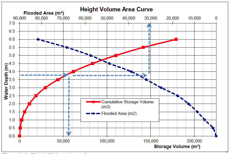
Figure 9-3: Height Volume Area Curve
As shown in Figure 9-3, a water depth of 3.75m would have a storage volume of 51,000 $m^3$ and a flooded area of 36,000 $m^2$. Alternatively, if 150,000 $m^3$ of storage is required, then the required water depth would be approximately 5.6m and the flooded area would be approximately 72,000 $m^2$.
9.3.2 Rough Estimate of Storage Capacity
During initial site visits it is often useful to establish an estimate of the site storage capacity before carrying out a detailed survey.
Stephens (1991) recommends the following equation for initial estimates of storage capacity.
Equation 9-2:
$\mathbf{Q = L \times T \times \frac{D}{6}}$
Where:
Q is the storage capacity [$m^3$]
L is the length of the dam wall at the full supply level [m]
T is the throwback (or fetch) of the reservoir [m] and measured in an approximately straight line from the wall.
D is the maximum water depth [m]
This figure is generally accurate to about 10% for the size and scale of dams covered in this document. L, T and D can all be estimated during a site visit with the use of an Abbney Level and an EDM.
9.4 Geotechnical Investigations
Geotechnical investigations will have to be carried out to establish the suitability of the foundation, abutments and spillway, any required foundation treatment, excavation volumes and slopes, and availability and characteristics of embankment materials. The investigations should cover classification, physical properties, location and extent of soil and rock strata, and occurrence and depth of groundwater within the foundation and reservoir area. Specifically the geotechnical investigations should yield information on:
- Depth, nature and condition of the bedrock along the dam axis and spillway. Bedrock that is close to the surface can present significant construction and/or seepage problems;
- Location of permeable layers along the dam axis which might cause excessive leakage or even piping failure under the dam;
- Identification of impermeable material along the dam axis into which the cut-off will be keyed into;
- Identification and assessment of suitable in-situ borrow material for dam construction;
- Location and assessment of ground conditions within the foundation area for stability, compressibility, and seepage.
9.4.1 Site Investigations
It is generally advisable to carry out investigations into the geological and foundation conditions of a dam-site for a depth equal to the height of the proposed dam. However, in view of the limited hydraulic heads dealt with in this publication and considering the generally high degree of consolidation of the soils in Kenya, it will in most cases be sufficient to investigate up to a depth of 4.00 metres. For dams with higher risks, considerable downstream infrastructure or questionable foundation materials, more detailed investigation will be required.
-
Bedrock
Bedrock at shallow depths should be detected and mapped. The weathered parts under the dam foundation and along the base surface of the cut-off trench will need to be removed. As this is an expensive exercise, possibly requiring blasting (which can further fracture the rock), it is therefore important to carefully assess the nature of the bedrock and whether it will need to be removed.
Heavily fractured bedrock can cause serious leakage and can be difficult to seal. Excavation of the fractured portion of the bedrock can be difficult and expensive to remove.
However, bedrock along the spillway axis, particularly at the sill cross section, is desirable, as this means that the channel may be less prone to erosion. bedrock along the spillway axis, particularly at the sill cross section, is desirable, as this means that the channel may be less prone to erosion.
-
Permeable Layers
All permeable layers, like gravel, murram, laterite and sand (old river-bed) under the dam and reservoir area should be detected as these can cause excessive seepage losses and potentially even cause dam failure. Mitigation measures (e.g. cut-off trench, clay layer, bentonite applications, synthetic lining etc.) can be included in the design if the presence of such permeable layers has been detected.
-
Foundation and Abutments
The foundation and abutment area requires ground conditions with stable soils. Ground conditions with soils of high organic content (e.g. peat), heavy swelling clays, saturated soils (swamps) or unconsolidated deposits are not suitable and the extent of unsuitable material should be mapped. A decision will need to be made as to whether the site is suitable, given these foundation conditions.
-
Access to Site
Access to site should be considered to ensure that the construction equipment can get to site. This may require an assessment of the roads and bridges that might be used by the construction equipment en route to the dam site itself.
-
Test Pits
Figure 9-4 shows a recommended type of test pit. Test pits should have a depth of at least 4.00 m, unless bedrock is struck before that depth. Test pits should be dug manually. Alternatively, the last two meters can be dug with the help of a hand auger. Test pits should be sized so that an engineer can enter the pit and examine the layers encountered. In general, a properly sized test pit will closely resemble the freshly excavated pit of a pit latrine.
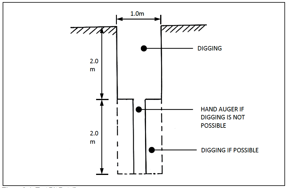
Figure 9-4: Test Pit Details
Figure 9-5 shows a tentative arrangement of test pits for a proposed dam. Along the dam axis test pits should be made at 10-15 metre intervals, and should be extended for approximately 30-50 metres horizontal from the expected upper contour level. Eight (8) more test pits should be made, four (4) upstream and four (4) downstream at 20-25 metre distances from the dam axis. The future centre-line of the spillway should be located as closely as possible and test pits should be sunk every 10-15 metres, in order to establish the position of the bedrock and to assess the suitability of the excavated material for construction purposes. Additional test pits should be located at any possible borrow areas and should be positioned to allow an initial estimate of available borrow volumes. To do this, a series of pits that establish the borrow area are needed. Their position and depths of suitable material can then be used for borrow volume estimations.
It is worth noting that Figure 9-5 shows 34 test pits which may seem excessive for a fairly small dam. Fewer pits can be used if there is confidence in the uniformity of the subsurface conditions. If this is the case, it should be noted in any survey reports. Final foundation details can be adjusted during core trench excavations. Test pits should be clearly numbered/named on the design drawings and when possible test pit logs should be digitally stored to allow easy access to the information they contain.
Uncovered test pits can present a danger to livestock, wildlife and humans. Test pits should be fenced off with brush or other materials when possible. Test pits should be back filled after examination if there is liable to be a significant period of time before construction begins.
Any test pits excavated in the reservoir area should be carefully backfilled with material which is watered and placed in shallow layers (150mm) and hand compacted such that the material has a density equal to the adjacent undisturbed soil.
Logs of the test pits should be established. Care should be taken to keep descriptions of the encountered materials as simple and understandable as possible. Figure 9-6 shows an example of a test pit log.
Samples of materials which will be submitted to the laboratory for testing (see Section 9.4.4) should be put in strong plastic bags, and marked with the (i) test pit number, (ii) depth at which it was taken, (iii) date at which it was taken. In general, samples of at least 20kg each are required for a full range of soil tests.
The results of the site investigations should allow the assessment of the suitability of the dam site with respect to the geology of the dam and reservoir area as outlined above. Reference is made to Section 9.6 where the basic geological requirements to be met are outlined.
Test pits on rocky sites should be carefully positioned to give as much information as possible with regard to both the soils and the rocky layers. In sites with large boulders, test pits that encounter boulders should be repositioned and re-dug.
-
Test Pits for Water Pans
The dimensions and purpose of test pits for water pans are exactly the same as test pits for dams. In the case of pans there is less concern with test pits under any embankments and more concern with test pits in the reservoir area. Test pits in the reservoir area should establish the types and quantities of soil to be excavated. If test pits expose pervious or porous layers, the depth to such layers should be noted so that the layers are not exposed during construction. For thin pervious layers, the depths to impervious layers below them should also be noted. For most small to medium sized pan projects, 15 to 25 test pits might be required to give a good feel for the subsurface conditions.
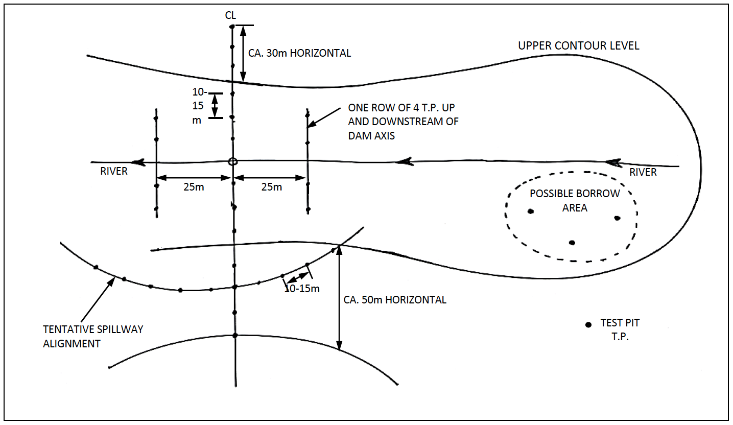
Figure 9-5: Site Investigations Test Pit Layout
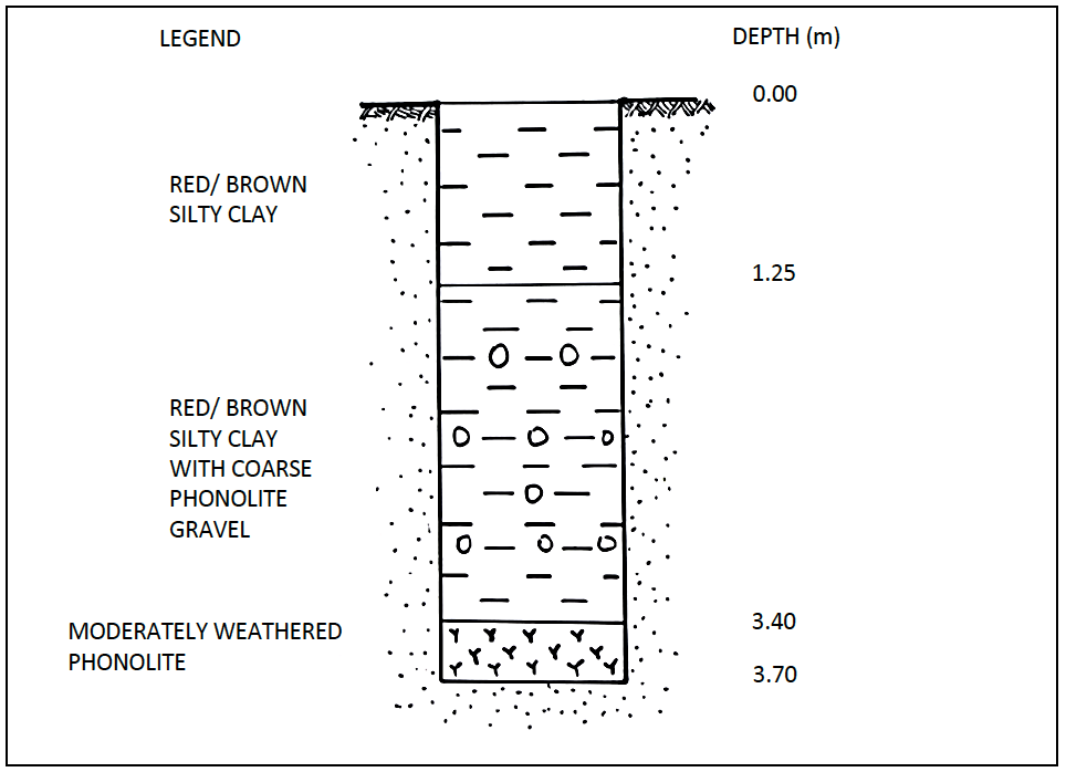
Figure 9-6: Test Pit Log
9.4.2 Availability of Construction Materials
Geotechnical investigations should establish the availability of construction materials.
-
Embankment Material
For reasons of economic feasibility, (see Chapter 11) suitable soil to be used as construction material should be available within a short distance from the dam site.
First the suitability of the material which will be excavated from the spillway should be investigated. Use of this material will mean a considerable economy on the construction cost. However, even when found suitable the quantity of material obtained from the spillway excavation may not be sufficient. Hence borrow areas for embankment fill material will have to be identified.
Borrow areas should preferably be located within the reservoir area, since removal of this material will increase the storage capacity. If this proves impossible, then borrow areas outside the reservoir should be identified. A few test pits (not less than four) should be dug in order to assess the suitability, depth, extent and homogeneity of the material. Initial borrow sources should be able to supply at least double the embankment fill volume. In general, it is not advisable to borrow clay material from the river bed just upstream of the embankment foundation as this can lead to exposure of pervious layers and lead to seepage problems.
Table 9-7: Soil Classification Chart (laboratory method)
CRITERIA FOR ASSIGNING GROUP SYMBOLS$^a$ GROUP SYMBOL GROUP NAME$^b$ COURSE GRAINED SOILS
More than 50% retained on No. 200 sieve (75mm micron)GRAVELS
More than 50% of coarse fraction retained on No. 4 sieve (4.75mm micron)CLEAN GRAVELS$^c$
≤ 5% finesCu ≥ 4 and
1 ≤ Cc ≤ $3^e$GW Well graded gravel$^f$ Cu < 4 and/or
1 > Cc > $3^e$GP Poorly graded gravel$^f$ GRAVEL WITH FINES$^c$
More than 12% finesFines classify as ML or MH GM Silty gravel$^{f,g,h}$ Fines classify as CL or CH GC Clayey gravel$^{f,g,h}$ SANDS
50% or more of coarse fraction passes No. 4 sieve (4.75mm micron)CLEAN SANDS$^d$
Less than 5% finesCu ≥ 6 and
1 ≤ Cc ≤ $3^e$SW Well graded sand$^i$ Cu < 6 and/or
1 > Cc > $3^e$SP Poorly graded sand$^i$ SANDS WITH FINES$^d$
More than 12% finesFines classify as ML or MH SM Silty sand$^{g,h,i}$ Fines classify as CL or CH SC Clayey sand$^{g,h,i}$ FINE GRAINED SOILS
50% or more pass sieve No. 200 (75 micron)SILTS AND CLAYS
Liquid limit less than 50inorganic PI > 7 and plots on or above line $A^j$ CL Lean clay$^{k,l,m,n}$ PI > 4 or plots below line $A^j$ ML Silt$^{k,l,m}$ organic $\frac{Liquid limit - oven dried}{Liquid limit - not dried} < 0.75$ OL Organic clay$^{k,l,m,n}$
Organic silt$^{k,l,m,o}$SILTS AND CLAYS
Liquid limit 50 or moreinorganic PI plots on or above Line A CH Fat clay$^{k,l,m}$ PI plots below line A MH Elastic silt$^{k,l,m}$ organic $\frac{Liquid limit - oven dried}{Liquid limit - not dried} < 0.75$ OH Organic clay$^{k,l,m,p}$
Organic silt$^{k,l,m,q}$Highly organic soils Primarily organic matter, dark in colour and organic odour PT Peat Notes
a Based on material passing No. 3 (75mm) sieve b If field sample contains cobbles and/or boulders, add “with cobbles and/or boulders” c Gravels with 5 – 12% fines require dual symbols GW-GM well graded gravel with silt GW-GC well graded gravel with clay GP-GM poorly graded gravel with silt GP-GC poorly graded gravel with clay d Sands with 5 – 12% fines require dual symbols SW-SM well graded sand with silt SW-SC well graded sand with clay SP-SM poorly graded sand l with silt SP-SC poorly graded sand with clay e $Cu = \frac{D_{60}}{D_{10}}Cc = \frac{(D_{30})^2}{D_{10} \times D_{60}}$ f If soil contains ≥ 15% sand, add “with sand” g If fines classify as CL-ML, use dual symbol GC-GM, SC-SM h If fines are organic, add “with organic fines” i If soil contains ≥ 15% gravel, add “with gravel” j If the liquid limit and plasticity index plot in hatched area on plasticity chart, soil is CL-ML, silty clay k If soil contains 15 – 29% plus No. 200 add “with sand” or “with gravel” whichever is predominant l If soil contains ≥ 30% plus No. 200, predominantly sand, add “sandy” m If soil contains ≥ 30% plus No. 200, predominantly gravel, add “gravelly” n PI > 4 and plots on or above line “A” on Plasticity Chart o PI < 4 or plots below line “A” on Plasticity Chart p PI plots on or above line “A” on Plasticity Chart q PI plots below line “A” on Plasticity Chart As outlined in Section 11.1, for dams over eight metres of height, where suitable soil is not available in sufficient quantities for constructing a homogeneous embankment, the construction of a zoned embankment can present a solution. In such cases, material excavated from the spillway could possibly be used as “random fill" for backfilling the shoulders of the embankment. It should however be noted that the design of zoned embankments should be carried out with due regard for the USBR filter criteria (United States Department of the Interior - Bureau of Reclamation, 1987).
-
Material for Drainage Blanket
The construction of a drainage blanket will require significant quantities for clean river sand and graded ballast. The source of the river sand should be determined and a sample taken for particle size analysis. In addition the source should be assessed to determine whether there are sufficient quantities and whether there are other competing interests for this sand (e.g. sand dams) that could cause a conflict or environmental degradation.
-
Material for Concrete Works
Most storage structures, although not all, require concrete to be used in various components of the structure (e.g. spillway sill, surround to draw-off pipe, ancillary structures, etc). Some consideration should be given to the availability of clean river sand and graded ballast in sufficient quantities for the proposed structures.
-
Water for Construction Work
Water is required for proper soil compaction, concrete works, and drinking water for the labour. Consideration should be given to the availability of water for the construction phase of the project as water trucking, if required, is an expensive undertaking. In general, during construction, an earth embankment will require a water volume equal to 30% of the embankment volume. Masonry and concrete structures will require less water but the importance of the water supply during construction cannot be overstated.
9.4.3 Soil Classification
The Unified Soil Classification describes different soil types by symbols as shown in Table 9-7.
A well graded soil implies that the soil has a fair proportion of all particle sizes. Conversely, poorly graded implies a soil with a significant proportion or excess of one soil type or particle size.
Silts and clays are further divided into those with low (L) and high (H) liquid limits. The Liquid Limit is the moisture content (water/dry weight soil %) at which the clay or silt becomes a slurry. A moisture content less than 50% denotes a low liquid limit. The liquid Limit is determined by the Atterberg Test (described in Section 9.4.4).
The Unified Soil Classification is presented in Table 9-7 together with the suitability of the soil for earth embankment dams shown in Table 9-8.
Table 9-8: Soil Suitability for Earth Embankments
| Group Symbol | Description | Soil Suitability for Earth Embankments | ||
|---|---|---|---|---|
| Homogeneous Dam | Zoned Dam | |||
| Core | Shell | |||
| GW | Well graded gravels | High | ||
| GP | Poorly graded gravels | Good/Fair | ||
| GM | Silty gravels | Good | ||
| GC | Clayey gravels | High | High | |
| SW | Well graded sands | High | ||
| SP | Poorly graded sands | Fair | ||
| SM | Silty sands | Fair | ||
| SC | Clayey sands | Good | Good/Fair | |
| ML | Inorganic silts with low liquid limits | Poor | ||
| CL | Inorganic clay with low liquid limits, also known as a “lean clay” | Good/Fair | Good/Fair | |
| OL | Organic silts or clays with low liquid limits | Not suitable | ||
| MH | Inorganic silts with high liquid limits | Poor | ||
| CH | Inorganic clay with high liquid limits, also known as a “fat clay” | Fair | Fair | |
| OH | Organic silts or clays with high liquid limits | Not suitable | ||
| Pt | Peat and highly organic soils | Not suitable | ||
The United States Department of Agriculture Texture Diagram (Figure 9-7) also provides a basis for classifying soil types based on the relative proportions of sand, silt and clay.
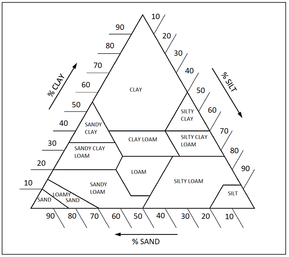
Figure 9-7: Soil Texture Class (USDA)
The USDA soil classes can be used for earth embankments as shown below.
Table 9-9: Texture Classes| Textural Class | % Sand | % Clay | Soil Suitability for Earth Embankments | ||
|---|---|---|---|---|---|
| Homogeneous Dam | Zoned Dam | ||||
| Core | Shell | ||||
| Loamy Sand | 70 – 85% | - | ✓ | ||
| Sandy Loam | 50 – 70% | < 20% | ✓ | ||
| Sandy Clay Loam | 45 – 80% | 20 – 35% | ✓ | ✓ | ✓ |
| Clay Loam | < 45% | 25 – 40% | ✓ | ✓ | |
| Sandy Clay | 45 – 65% | > 35% | ✓ | ✓ | |
| Clay | < 45% | > 40% | ✓ | ||
(Source: Stephens, T. 1991)
Generally silts are unsuitable as embankment fill material due to their inherent instability when wet.
The description of soil should provide the following information:
- Name and symbol
- Percentage of gravel, sands and fines
- Colour in moist condition;
- Perviousness or drainage properties;
- Plasticity characteristics;
9.4.4 Soil Tests
-
Visual and Field Tests: A number of simple tests which can easily be carried out in the field permit a preliminary evaluation of the prospective fill material's suitability.
-
With the naked eye a first classification of the available materials can be made. Heavy clays and soils containing an excessive percentage of sand can be identified and classified as unsuitable. Heavy clays are subject to considerable swelling, shrinking and cracking, while soils containing too much sand are in general too permeable.
Soils in which most particles are visible to the naked eye are generally too sandy and should also be classified as unsuitable for homogeneous dam construction. Soils with hardly any particles visible to the naked eye (heavy clays) should be treated carefully and submitted to laboratory tests to assess their suitability for homogeneous dam construction.
Consequently, soils with around half (50%) of all particles visible to the naked eye are generally suitable for homogeneous dam construction.
- To establish the existence of cohesion, add roughly 10 % of water (volume) to a soil sample, mix, and proceed as follows:
- Soils which cannot be rolled into a ball without breaking up are either too sandy or have a highly irregular granular distribution. These soils should be avoided. Alluvial deposits of fine sand and silt may demonstrate this feature.
- Soils which can be rolled into relatively thin threads (diameter approximately 8 mm) without breaking up contain a high proportion of clay. Consequently suitable soils are those which can at least be rolled into a ball but no further than a thread with ±8 mm diameter and ±150 mm of length, before it starts breaking into pieces. A wet clay will also exhibit a shiny smooth surface when cut.
- Dry silts are similar in appearance and feel to wet clays but unlike clays which exhibit sticky, plastic like properties, a wet silt has a silky, smooth feeling. Silts do not make good embankment material unless mixed with other soil types (clays and sands).
- It should be confirmed that the soil is not rich in organic matter. Usually, organic soils can be distinguished from the inorganic by their characteristic odour and their dark-grey or black colour.
- The dilatancy or shaking test can indicate the degree of plasticity. The wetted soil is formed into a pat on the open palm of the hand. The hand is shaken horizontally. If water comes to the surface making it glossy, the sample should be squeezed between fingers and the gloss should disappear. A reaction that is rapid indicates lack of plasticity and no reaction indicates a highly plastic clay which is also unsuitable.
- In situ permeability tests can be carried out to determine the permeability of soils at the dam site. A rough falling head permeability test is described below.
- Dig or bore (with an auger) a suitable hole in the ground at the dam site. The hole should extend below the topsoil layer. If using an auger, a depth of 2 to 3 meters is desirable.
- Measure the hole sufficiently to determine the wetted surface area when it is filled with water.
- Fill with water and observe how quickly the water level drops. Keep track of elapsed time. Top up as needed to maintain the water level. Ideally this should be done over a period of several hours to ensure that the surrounding soil becomes saturated.
- In the final 30 minutes, observe the drop in water level over a period of time and then top up with water and measure the volume used to top up.
- A rough permeability can be calculated by taking the top up volume divided by the wetted area and then dividing the result by the time observed in step d. The result can be expressed in mm/s and should be in the range of 1 x 10⁻⁴ mm/s.
- In the event of very permeable soils and community projects it is advisable to get the community to observe the in situ permeability testing so they fully understand the scale of possible seepage losses.
-
-
Laboratory Tests: The purposes of performing laboratory tests on soil samples in relation to design and construction of small dams are:
- Assessment of suitability of foundation and construction material, and
- Monitoring of compaction during the construction of the embankment.
The taking of “undisturbed" samples from test pits will in general require the services of specialised operators. Disturbed samples in plastic bags can be obtained as mentioned under Section 9.4.1. The performance of the following tests is highly recommended for the assessment of prospective construction materials. These tests can be performed at approved soil testing labs within the country. Services can be obtained from higher learning institutions, Ministry of Public Works, national research facilities (e.g. KARI, KALRO) and certified private soil testing laboratories: More information on specific tests can be found in British Standard BS1377 or in Eurocode EN1997.
-
Particle Size Analysis: This test is used to determine the type of soil. The test is carried out by means of sieving (and for the finer fractions by sedimentation). Basically, the soil sample is passed through a series of standard test sieves having successively smaller mesh sizes. The results of this test are represented as a curve on a semi-logarithmic plot, the ordinates being the percentage by weight of particles smaller than the size given by the abscissa (Figure 9-8). Soils suitable as construction materials for homogeneous small dams are generally represented by a smooth concave distribution curve.
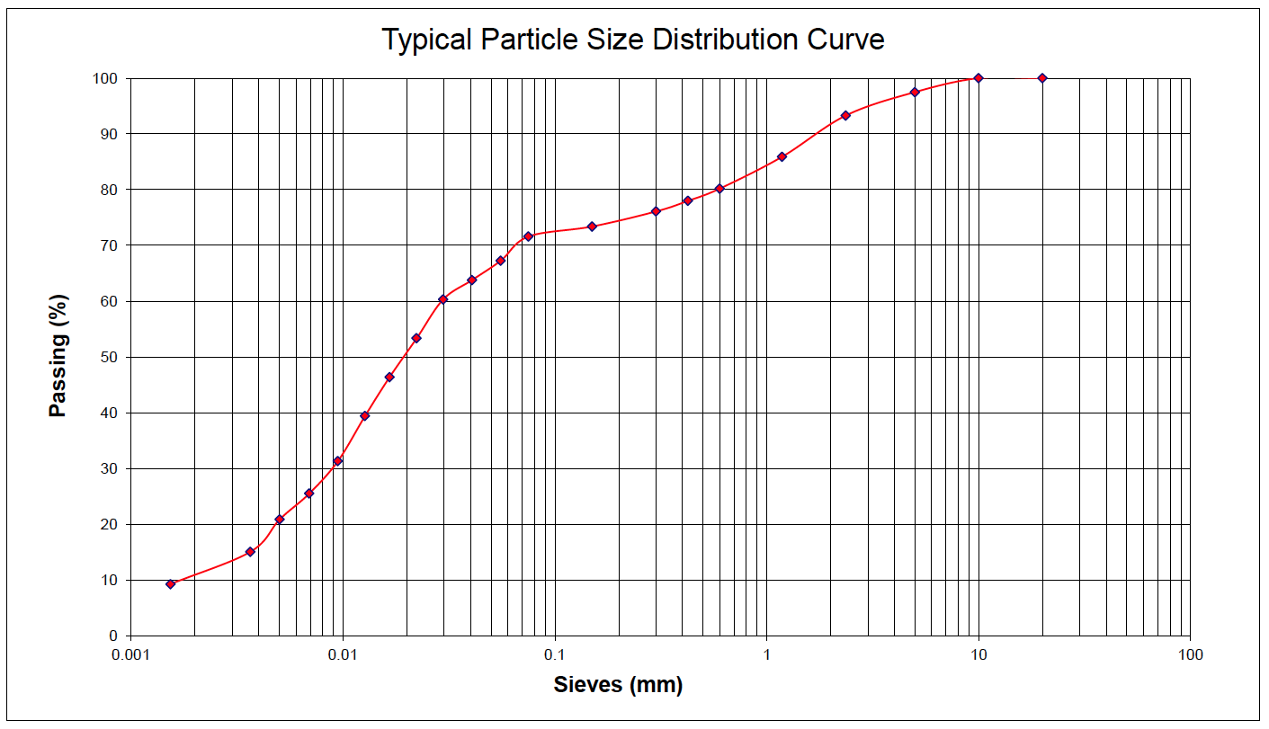
Figure 9-8: Particle Size Distribution
-
Atterberg Limits: Depending on its water content a soil may exist in the liquid, plastic, semi-solid or solid state. The water contents at which the transitions between states occur vary from soil to soil. Most fine-grained soils exist naturally in the plastic state. The upper and lower limits of the range of water content over which a soil exhibits plastic behaviour are defined as the liquid limit ($W_L$) and plastic limit ($W_P$) respectively. The water content range itself is defined as the plasticity index ($I_P$ = $W_L$ – $W_P$). The transition between the semi-solid and solid states occurs at the shrinkage limit, defined as the water content at which the volume of soil reaches its lowest value as it dries out.
It has been observed that many properties of silts and clays, can be correlated with the Atterberg limits by means of the plasticity chart (Figure 9-9).In general soils that fall above the “Line A” in Figure 9-9 and have a liquid limit ($W_L$) above 30% are suitable:
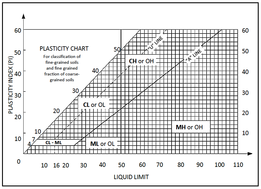 Figure 9-9: Plasticity Chart
-
Proctor Compaction Test: This test will determine the optimum water content, and the corresponding maximum dry density of the soil which can be obtained for a particular compactive effort. Figure 9-10 shows a typical (dry density/water content) relationship.
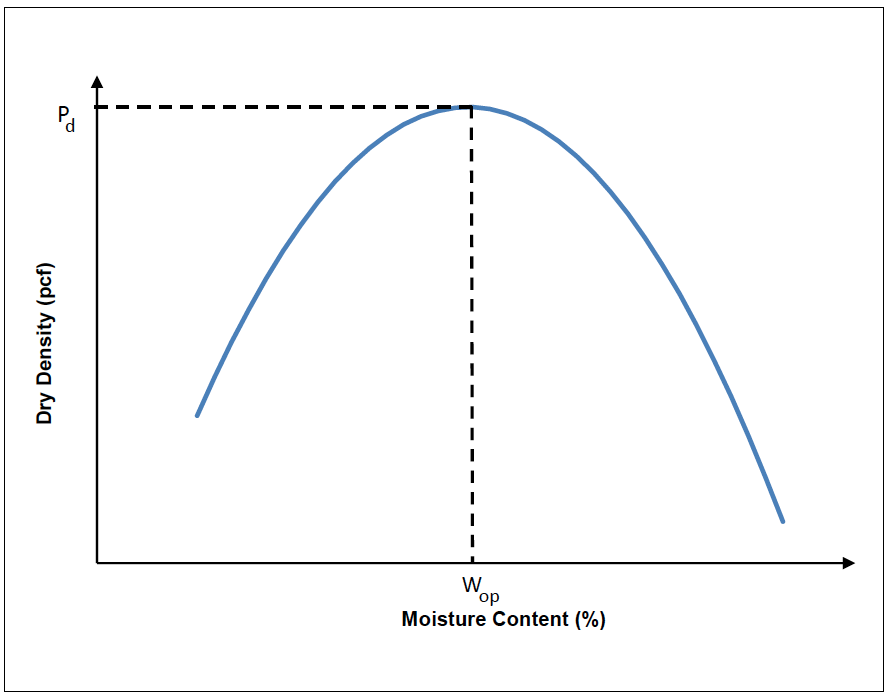 Figure 9-10: Proctor Curve
A minimum construction requirement of 95% to 100% of the maximum dry density obtained in the Proctor test is usually specified.
Test procedures concerning the above laboratory soil tests are described by Craig (Knappett & Craig, 2012) pp. 26-29. The tests can be performed on disturbed samples.
-
Dispersivity: Soils which are to be used as construction material should systematically be tested for dispersivity. The use of dispersive clays as construction material has caused many failures of small dams in Kenya and elsewhere. Dispersivity can be defined as post-construction de-flocculation of clay, which leads to a complete loss of tensile strength. Dispersive characteristics of soils are generally closely related to the exchangeable sodium percentage (ESP). If the ESP value is higher than 8 %, the soil may be dispersive. An ESP value of 5 % or less can be considered safe. In cases of doubt a crumb test can be performed: in this test a cube of soil is placed in a dish of de-ionised water, and the tendency of colloidal-size particles to de-flocculate and go into suspension is closely observed.
For higher risk structures (taller walls, downstream infrastructure, etc) the performance of more advanced tests to determine the shear strength parameters (cohesion; friction angle) of the prospective construction material should be considered. These tests are necessary for any sort of foundation and slope stability investigations. Reference is made to Craig (1983) for any inquiries concerning these tests.
9.4.5 Typical Soil Properties
Typical soil properties are presented in Table 9-10 which provides a guide to cross check laboratory results.
Table 9-10: Average Soil Properties for Different Soil Types
| Soil Group Symbol | MDD (Kg/$m^2$) | OMC (%) | Cohesion (Kg/$m^2$) | Tan | Permeability (cm/sec) |
|---|---|---|---|---|---|
| GC | > 1840 | <15 | N/A | > 0.60 | $10^{-6}$ to $10^{-8}$ |
| GM | > 1830 | <15 | N/A | >0.67 | $10^{-3}$ to $10^{-6}$ |
| SM | 1830 ± 16 | 15 ± 0.4 | 500 ± 500 | 0.58 ± 0.07 | $10^{-3}$ to $10^{-6}$ |
| SC | 1840 ± 16 | 15 ± 0.4 | 1100 ± 600 | 0.6 ± 0.07 | $10^{-6}$ to $10^{-8}$ |
| ML | 1650 ± 16 | 19 ± 0.7 | 900 ± NA | 0.62 ± 0.04 | $10^{-3}$ to $10^{-6}$ |
| CL | 1730 ± 16 | 17 ± 0.03 | 1200 ± 200 | 0.54 ± 0.04 | $10^{-3}$ to $10^{-6}$ |
| CH | 1510 ± 32 | 25 ± 1.2 | 1300 ± 600 | 0.35 ± 0.09 | $10^{-6}$ to $10^{-8}$ |
| MH | 1310 ± 64 | 36 ± 3.2 | 2000 ± 900 | 0.47 ± 0.05 | $10^{-4}$ to $10^{-6}$ |
10 Reconnaissance Survey
The reconnaissance survey is an important component of the project assessment. This activity compliments the project planning exercise and should be conducted properly to ensure as much information pertinent to the project is identified and collected (See also Chapter 3 - Project Planning and Management). Preliminary ESIA screening and scoping can also be conducted during this stage.
A reconnaissance survey should take place early in the project planning. It will help to:
- determine the suitability of a storage project to address water supply problems;
- determine the best embankment or reservoir options;
- establish catchment size and initial water availability and historical flood marks;
- establish other areas of concern.
10.1 Desk Study
This will involve assessment of primary and secondary sources of information relevant to the proposed survey area, including maps (topography, satellite, vegetation, soils, etc.) and reports from similar works done. The desk study must provide preliminary insight on the suitability of the proposed site, before proceeding to site. A second desk study will almost always be needed after the site visit as well.
10.2 Site Identification
Site identification can involve many different criteria depending on the type of storage to be constructed. The following section applies mainly to earth embankments but can also be applied to other types of storage as well. It cannot be stressed enough that an accurate GPS position for the proposed site should be recorded. The position and map datum that the GPS uses can then be used to locate the site accurately on existing contour maps, Google earth and other software/mapping programs.
The general considerations that must be considered for all storage sites include:
- Location of final water use;
- Size of catchment and available inflows;
- Site topography;
- Geology of the dam and reservoir areas;
- Availability of construction materials;
- Spillway location considerations;
- Sedimentation;
- Evaporation;
- Settlement in the area and potential settlement or resettlement requirements;
- Risks to downstream inhabitants;
- Other storage structures in the area;
- Land ownership.
10.3 Tools and Equipment for Reconnaissance Survey
Table 10-1 suggests tools and equipment that the reconnaissance team can use during the initial visit. Other more basic field items that could assist the team should be considered. These include gumboots, umbrellas, hats, sunscreen etc. Spare batteries for all equipment should be carried. If the field visit is in a remote area, battery charging equipment should be carried for computers and other equipment.
Table 10-1: Tools and Equipment for Reconnaissance Survey
| Tool/Equipment | Function |
|---|---|
| Camera | Capturing still images of survey area |
| GPS | Collecting geospatial information; elevations, location etc. A variety of handheld GPS units are available in Kenya. They can be set to a variety of reference datums and units. They can record positions very accurately but are less reliable for elevations. In general if a handheld GPS is showing a positional accuracy of ±3m the elevation accuracy is ±30m. More advanced GPS units can measure areas and distances very accurately. |
| EDM | Collecting distance measurements. Modern EDMs can measure distances up to about 1,000m without the need for specialized survey reflectors. Typical high end EDMs come with an inclinometer and can measure angles of inclination (usually within a ±30 degree range). EDMs with inclinometers can be used to calculate vertical heights with the use of basic trigonometry. |
| Abney Level | Measuring angles of inclination/ slopes between points |
| Sample Bags and Labels | Collecting and identifying soil samples |
| Maps | Identifying locations, features etc. within survey area. In general 1:50,000 topographic maps for most areas in Kenya are available. These are a reasonable scale for determining catchment areas but are not detailed enough for any sort of storage estimations. In Northern Kenya, only 1:100,000 maps may be available. For large projects and large catchments areas 1:250,000 maps of the entire country are available. |
| Spade, hoe, machete (“panga”) | Collecting soil samples |
| Water Bottle | Collecting water samples for analysis and conducting field soil tests. |
The list above is by no means exhaustive and additional more specialized equipment may be required.
10.4 Selection of Appropriate Type of Structure
For reservoirs located along water courses, the main options and considerations for storage structures are summarised in Table 10-2 below:
Table 10-2: Considerations for Structures on Water Courses
| Storage Structure | Considerations |
|---|---|
| Earth Embankment | Valley side slopes (must be gentle enough to allow machinery access). Impermeable foundations capable of supporting the embankment. Availability of borrow material. Suitable spillway locations away from embankment (i.e. gentle side slopes on at least one side of the valley where a spillway can be excavated). |
| Mass Gravity Walls | Type of foundation materials (usually require firm rock foundations and rocky valley side slopes). Availability of construction materials. Suitable spillway locations along valley side slopes. Relatively low water depths (generally less than 5m for small structures). |
| Sand Dams | As with mass gravity walls above but in a valley with large sand/sediment loads, construction will be carried out over several rainy seasons. Suitable solid and impermeable banks into which the wall can be anchored. |
| Subsurface Dams | Wide, permeable valleys with significant subsurface flow or sub surface water holding capacity. Suitable subsurface rock surface or solid impermeable foundation on which the wall can be constructed. |
For reservoirs located outside of water courses, the main options and considerations for storage structures are shown in Table 10-3:
Table 10-3: Considerations for Structures Not on Water Courses
| Storage Structure | Considerations |
|---|---|
| Pans | Flat or gently sloping (max 3%, best 1%) ground, may have an existing natural depression. Deep soils that can be excavated and the ability to direct surface runoff into the structure. |
| Lagoon | Sloping ground (up to 10%) Suitable borrow material within the reservoir area for construction of embankment walls on the low sides of the site. Ability to direct surface runoff into the structure. |
| Rock Catchment | Suitable rock face for collecting runoff (gently sloping with topography that allows runoff capture with low training walls). Suitable area for tank or gravity wall construction to store water. |
10.5 Location of Final Water Use
In principle, the reservoir site should be located reasonably close to the area where the stored water will be used as this reduces the cost of conveying the water to the supply area. In addition if the topography allows, the option of a gravity supply from the reservoir to the supply area should be considered.
10.6 Size of the Catchment Area and Available Inflows
The size of the catchment has a bearing on (i) inflow into the site, (ii) size of spillway and required freeboard and (iii) rate of sedimentation. Consequently it is not economic to put a small dam on a large catchment. Furthermore a catchment area that is too small for the proposed storage structure may result in insufficient inflow.
Catchment size and expected inflows are discussed in detail in Chapter 8 on hydrology.
For a quick estimation of inflows, Equation 10-1 can be used.
Equation 10-1:
$\mathbf{Q = C \times A \times R \times 1000}$
Where:
Q is the annual inflow [$m^3$/year]
C is runoff coefficient. A value of 5% (dry year) to 20% (normal) can be used
A is the catchment area [$km^2$]
R is the annual rainfall [mm]
10.7 Topography of Dam Site
Ideally, a dam site should be located in a narrow part of the river, just downstream of a relatively wide stretch (See Figure 10-1). The dam should be located in a stretch of the river which has a flat longitudinal slope. This will generally allow the best storage option without excessively tall embankments. Although a variety of alignments can be tried, the best alignment is usually perpendicular to the watercourse. If the axis cannot be positioned at the narrowest point on the river course, then the next best options are on the upstream part of the constriction (i.e. as the valley narrows).
An important factor in assessing the economic suitability of a prospective earth dam site is the storage ratio (water storage volume / earth fill volume). Sites where the storage ratio is below 3 (poor) to 5 (moderate) should, in fact, not be considered. A good site should offer a storage capacity / earth fill ratio of at least 8 (fair) to 15 (good).
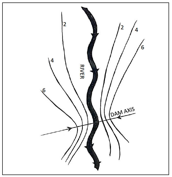
Figure 10-1: Topographic Location of Dam Axis
10.8 Topography of Pan Sites
In general pans are best suited to sites that are flat or very gently sloping (1% to 3% slopes work best). For rectangular pans, the long side of the pan should be positioned parallel to the contour lines. This will result in the minimum earthworks required for any embankments and will ensure that the pan can capture surface runoff.
10.9 Geology of Dam and reservoir Area
Two basic requirements are to be considered concerning the geology of the dam and reservoir area.
10.9.1 Embankment Foundation
At the location of the embankment, the foundation material should be firm enough to carry the weight of the dam wall. Care should be taken in detecting the presence of any sand layers in the foundation area, since this can cause excessive seepage. In general, for earth embankments less than five metres in height, the risk of embankment failure through piping - washing out of small soil particles because of uplift pressure in the downstream area of the embankment - is not very serious, due to low water heads.
10.9.2 Water-tightness of the Reservoir
In sandy areas, heavy losses of water from the reservoir through infiltration and/or leakage (on top of the evaporation losses) will render the construction of the dam unviable. Therefore, in such areas, construction of surface water storage facilities without lining should, as a rule, not be recommended.
Technical solutions for excessive water losses through infiltration can be found and include clay lining, soil additives (bentonite or similar) or lining with HDPE or LDPE lining materials. In general, the use of lining materials only makes economic sense where the stored water is being used for commercial production.
10.10 Availability of Construction Materials
Suitable construction material (soil) should be available in sufficient quantities within a short distance from the dam site, preferably within the reservoir area since this will increase the storage capacity. Lack of suitable construction material within an acceptable distance from the dam site can render the construction of a dam at an otherwise good site completely uneconomical.
Construction material considerations should not be limited to suitable earth embankment materials but should also examine availability of water, sand, ballast and hardcore.
Water will be needed for proper compaction. Generally a water volume of 25 to 30 percent of the embankment volume will be needed.
If heavy equipment is to be used, both access roads and availability of fuel and oil must be considered.
10.11 Site Accessibility for Construction
Issues for consideration would include availability and loading capacity of river crossings, height restrictions, and road orientation in the case of low loaders.
10.12 Possibilities for Spillway Location
For the type and size of dams under consideration, it is usually not economically viable to incorporate large concrete structures (such as spillway channels, culverts, earth retaining walls etc.) into the design. In order to avoid the need for such structures, the following should be kept in mind, while assessing prospective dam sites:
- The spillway should be kept away from the embankment in order to minimise the need for protection structures (retaining walls);
- Steep valleys should be avoided, since they will either require a concrete sill (due to high water velocity), or excessive excavation (the length of the spillway will have to be increased) in case an earth channel spillway is used.
With regard to spillway placement, the preferred sites are narrow valley stretches with relatively steep sides up to the required water level, above which at least one of the valley embankments flattens considerably (Figure 10-2).
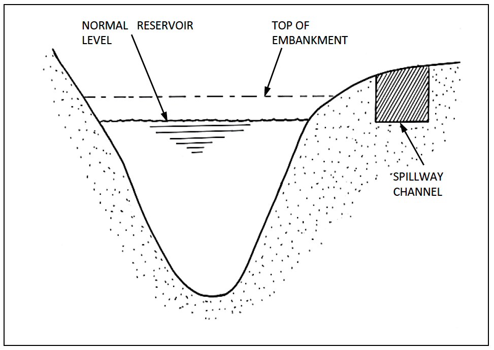
Figure 10-2: Spillway Location Possibilities
10.13 Sedimentation
Sedimentation is discussed in Chapter 8 (Hydrological and Sediment Analysis). In general, sedimentation from large catchments can be very problematic in Kenya. The size of catchment, land use in the catchment and existing evidence of erosion or large sediment loads should be noted.
Often, offline storage (storage constructed off the main river or lagga channel) is preferable from a sedimentation viewpoint. In such cases, inlet channels/structures can be constructed to allow water inflow from the main catchment when sediment conditions are the most favourable (toward the end of the rainy season).
10.14 Evaporation
Evaporation is discussed in Section 3.3.10 and Chapter 8 (Hydrology) and should be considered during the reconnaissance survey. Evaporation losses from reservoirs with large surface areas can be excessive. In general, shallow reservoirs with large surface areas should be avoided in areas with high evaporation.
10.15 Land Ownership
Land ownership and sample agreements for storage construction are discussed in detail in Section 4.5. Ownership of the dam and reservoir area (or other storage structure) should be thoroughly sorted out as soon as a suitable construction site has been selected. Cost of land compensation and/or resettlement of people might be forbidding or might upset the economic viability of the project.
In the case of a dam, enough land should be set aside, not only to cover the dam and reservoir area, but also for the spillway channel and other ancillary structures, as well as for possible borrow areas outside the reservoir. Sufficient allocation of land for other water conservation structures should also be considered.
The social impact on the affected landowners and communities should also be taken into account for each considered dam site, and sites where the consequences of resettlement or loss of valuable (fertile) land are considered important should be avoided.
As early as possible in the planning and design process, land issues should be addressed and resolved by the community with the possible assistance of the County Lands Office.
For smaller, more commercially oriented storage, it is important to note that rivers and laggas often form property boundaries and it can be difficult to get agreement from property owners on both sides of the stream or lagga.
10.16 Risk Assessment
Potential risks due to the proposed project should be identified and assessed. Fatal flaws, or issues that can cause unanticipated problems should be pre-empted and possible solutions identified. At this stage of the project, the risk assessment will mainly examine what sort of “deal breakers” exist and how likely they are to become serious issues.
10.17 Desk Study (Part II)
At the conclusion of the reconnaissance visit, it is usually beneficial to undertake a second desk study. Maps and reference materials that were mentioned during the visit can be located and used for additional planning. Consultation with other actors can be undertaken, including the local county water office if appropriate.
10.18 Reconnaissance Visit Reports
A brief report on the reconnaissance visit is recommended. It should cover all of the topics listed above and it should make a recommendation as to whether the proposed site should or should not be considered for storage development. If the site should be considered for storage development, the report should highlight any emerging issues that require further investigation.
A proposed reconnaissance visit report outline is provided in Chapter 19.
11 Feasibility Study
A feasibility study for small scale storage looks at most of the same issues that the full design addresses. The main difference between the feasibility and design reports are that the feasibility report looks at a broader selection of options and does not address the same level of detail that the design report covers once a recommended option has been agreed upon.
In general, the field work required for a feasibility report is the same fieldwork required for a full design. This includes a complete survey of the site as well as visits throughout the catchment and downstream areas.
The following sections describe the steps that should be taken when conducting a feasibility study for a proposed site. They are laid out to match as closely as possible the feasibility study reporting format set out in Chapter 19.
11.1 Executive Summary
This should be a brief (one page is normally sufficient) description of the project. It must state the background and purpose of the project. It should summarize the expected costs, the beneficiaries and the technical details of the project. It should present any viable alternatives and lay out the way forward.
11.2 Background and Purpose of the Proposed Storage Structure
The proposed project should be fully described in the report.
11.2.1 Stakeholders
An assessment should be made of the project stakeholders and contact details of relevant people (owners, managers, caretakers, local WRUA, etc) should be obtained.
11.2.2 Purpose of the Project
The feasibility report should clearly state the purpose of the project (e.g. to store 20,000 cubic meters of water in a pan to increase the time when grazing can occur in the sub-location). The purpose must be attainable by the proposed project.
11.2.3 Location
The location of the proposed project should be correctly identified and detailed. This includes land registration details where available, ownership details, GPS coordinates and datum. This information will be used to develop the relevant layout maps. Ideally, at least two maps should be produced. One should show the proposed storage location and the extents of the catchment area and the other should show the site layout that shows possible dam alignments and flooded areas.
Details of the county, sub-county, location and sub location should be captured, as well as a summary of how to access the site. This information will be included in the feasibility report.
11.2.4 Details of Site Visits
The report should show the time frame for site visits, identify who went to site and identify who was contacted in the project location.
11.3 Analysis of Alternative Options to Meet Project Objectives
This should briefly touch on what other alternatives exist that might also meet the project objectives. It does not have to examine the alternatives in detail but it must give sufficient details to explain why they are not being considered as a way forward.
11.4 Analysis of Water Demand
The study should look at the expected water requirements. Expected water use figures for a variety of design options can be found in Section 3.3 of this document.
For specialized water use or requirements, the details should be clearly captured and documented in the feasibility report.
11.4.1 Offtakes and Other Structures
This will involve the identification of possible sites for offtakes, community water points, cattle troughs, pump houses, fencing and other associated structures. These points can be mapped out and detailed on the layout map submitted in the feasibility report.
This section is mainly to help finalize cost estimates. Final details and drawings for offtakes and structures will be concluded in the design process.
11.5 Site Investigations
Details should be given on the site topography and on the soils and geotechnical information. If additional information is required for the design it should be identified here.
11.5.1 Impoundment Area Details
A full survey of the impoundment area will be required. This will also include identification and marking out of the possible locations of dam components (spillway, embankment, etc…). A contour map of suitable scale should be produced. Various dam alignments and heights can then be considered to produce a selection of possible storage options.
Survey data and contour maps for each option should be included in the report. Section 9.1 provides details on the intensity of survey points and survey beacons.
If relevant, the site maximum site storage should also be presented.
11.5.2 Results of Geotechnical Investigations
The results of any geotechnical investigations should be presented. At a minimum these should include test pit details and borrow material details, plus the laboratory analysis of the soils sampled from the test pits.
This section should also identify any further investigations that may be needed as part of the final design.
11.5.3 Recommended Storage Structure
Details of the recommended storage structure should be given along with justifications for choices.
11.6 Environmental and Social Considerations
Any emerging environmental considerations should be identified and examined during this phase. Essentially, the feasibility study provides an opportunity to scope out the work involved in conducting the Environmental and Social Impact Assessment, as described in Chapter 6.
In arid areas, special attention should be paid to grazing concerns and the potential for human/wildlife conflict.
In more built up areas, the risk of failure of the embankment on downstream settlements and/or developments should be examined.
Any resettlement or other legal issues that may arise as a result of the project should be identified at this point.
11.7 Hydrological Analysis
The full hydrological analysis for the project should be carried out during the feasibility stage. Refer to Chapter 8 for details.
11.7.1 Inflow Estimation
Catchment details should be determined. They should include catchment area, soil types, vegetative cover and catchment condition. Catchment elevations and flow path elevation and length details should be determined.
Inflows for the dam should be estimated. This can be done based on general annual rainfall averages, on monthly or daily stream flow or on monthly or daily rainfall data. See Section 8.8 for further details.
All data (and their sources) should be recorded in the report.
11.7.2 Reservoir Simulation or Modelling
Reservoir simulation can be carried out based on the storage options, the expected water use, the estimated inflow estimations, as well as the evaporation and seepage estimates. This is discussed in Chapter 8 and can be done graphically, via spreadsheet calculations or via commercial software.
The result of the reservoir simulation is to examine a selection of storage options to determine which option best fits the inflows and water use.
11.7.3 Estimated Spillway Sizes and Inflow Design Flood
In order to produce a cost estimate as part of the feasibility study, a spillway design must be carried out. At this stage, it is sufficient to base the spillway design on an estimated flood based solely on the catchment area. Table 8-6 provides general guidelines for design flood estimation based on catchment area.
Once a design flood has been estimated, initial estimates of spillway details (width, depth, alignment, etc) can be calculated and presented in the report. Table 11-1 gives preliminary estimates for required spillway widths for a variety of design floods and approach heights. The widths have been calculated based on the broad crested weir formula.
Table 11-1: Spillway Widths for Various Design Floods and Approach Heights
| Design Flood ($m^3$) |
Required Width for 0.5m Approach Depth (m) |
Required Width for 1m Approach Depth (m) |
Required Width for 1.5m Approach Depth (m) |
Required Width for 2.0m Approach Depth (m) |
|---|---|---|---|---|
| 5 | 9 | N/A | N/A | N/A |
| 10 | 17 | N/A | N/A | N/A |
| 15 | 25 | 9 | N/A | N/A |
| 20 | 34 | 12 | N/A | N/A |
| 25 | 42 | 15 | N/A | N/A |
| 30 | 50 | 18 | 10 | N/A |
| 40 | 67 | 24 | 13 | N/A |
| 50 | 84 | 30 | 16 | 11 |
| 75 | 126 | 44 | 24 | 16 |
| 100 | N/A | 59 | 32 | 21 |
| 150 | N/A | 89 | 48 | 32 |
| 200 | N/A | 119 | 64 | 42 |
| 250 | N/A | 147 | 80 | 52 |
| 300 | N/A | 177 | 96 | 63 |
11.7.4 Sediment Inflow
Sediment inflow should be estimated as laid out in Section 8.13. Sediment inflow will affect the life span of the dam. The NWMP 2030 suggests the following design criteria for water supply infrastructure:
- Rural = 20 yrs
- Urban = 50 yrs
11.8 Identification of Design Issues
Identification of design issues that will be addressed during the full design should be mentioned in the feasibility report. In general, they will involve revising spillway dimensions, finalizing offtake arrangements, determining details on ancillary structures, and additional modelling that might be necessary for larger projects, etc.
11.9 Construction Plan
A project construction plan should be developed. It should present tentative time frames for design work, any necessary social interventions, NEMA and WRMA approvals, actual construction period and a tentative date for completion of works.
A critical path analysis can be included to emphasize the key steps that must be achieved.
11.10 Cost Estimate
The feasibility study must present a cost estimate for the project. The cost estimated should be based on expected construction costs and calculated from a preliminary bill of quantities for the project.
In general, in 2014, construction costs of small scale water storage in Kenya ranged from Ksh. 50 per cubic meter to over Ksh. 500 per cubic meter of water stored. The lowest costs are usually seen in large reservoirs (500,000 to 1,000,000 $m^3$ of storage) while the highest costs are usually seen in smaller reservoirs. (5,000 to 20,000 $m^3$ of storage). These figures are based on construction experience in Kenya over the last 10 years and compare well with the NWMP 2030 estimate of Ksh. 333 per cubic meter for small dams.
11.11 Economic and Financial Considerations
The feasibility study should look at the expected cost of the project and compare it to alternative options and average costs in Kenya. A cost per beneficiary can be established and compared against the alternative options. Cost per beneficiary for a variety of alternative options can be established from the Project Unit Costing, WSTF, and (June 2011) or from the NWMP, 2030. A cost/benefit analysis should be conducted even if the scale of the project and the detail at this stage does not warrant a detailed analysis. However the total project cost, covering design, construction, supervision, and all environmental and social mitigation measures can be estimated. This may not reflect the true cost of all the impacts but assumptions regarding the estimation process can be described.
The benefits of the project should be described and estimated and compared to the costs. The intention is to avoid making investments in projects that cannot be justified due to the cost. The willingness and ability of project beneficiaries to pay (or assist in paying) for the proposed project should be stated.
11.12 Project Financing
The feasibility report should identify possible financing sources and raise any financial issues that may affect the project.
11.13 Analysis of Risks and Proposed Mitigation Measures
Results of any risk analysis work should be included. If mitigation measures have been identified, then details should be provided. If no mitigation measures have been finalized, then the report should describe in detail what work still needs to be carried out to ensure that the project can move forward.
11.14 Conclusions
The conclusions should address:
- Legal, Social and Environmental feasibility;
- Technical feasibility;
- Financial details/feasibility;
- Economic Feasibility.
They should be clearly stated in the executive summary.
11.15 Recommendations
The recommendations should summarize:
- Measures required to enable the project to meet its objectives;
- Way forward.
They should be clearly stated in the executive summary.
11.16 Annexes to the Feasibility Report
There is often a long period between the initial feasibility report and the implementation of the project. Social, environmental and legal issues must be dealt with, financing must be secured, and other government approvals must be obtained. In order to keep continuity between the feasibility work and any future design work, it is strongly recommended that the feasibility report has annexes with site photos and all relevant maps. These can be extremely important for refreshing memories and for introducing new team members to the project.